import time

from IPython.display import HTML
from itables import to_html_datatable
from joblib import Parallel, delayed, cpu_count
import numpy as np
import pandas as pd
import plotly.express as px
import scipy.stats as st
import simpy
from sim_tools.distributions import ExponentialParallel processing
Learning objectives:
- Learn how to implement parallel processing.
- Understand how to choose an appropriate number of cores.
Relevant reproducibility guidelines:
- STARS Reproducibility Recommendations: Optimise model run time.
Pre-reading:
This page continues on from: Replications.
Entity generation → Entity processing → Initialisation bias → Performance measures → Replications → Parallel processing
Required packages:
These should be available from environment setup in the “Test yourself” section of Environments.
library(data.table)
library(dplyr)
library(future)
library(future.apply)
library(ggplot2)
library(knitr)
library(plotly)
library(simmer)
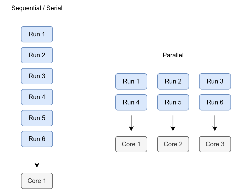
library(tidyr)A computer’s processor has multiple cores. Each core is like a worker that can do tasks.
Normally, when you run a program, it only uses one core, so only one worker is doing the job. This is referred to as serial or sequential processing.
Parallel processing means telling the computer to use more than one core at the same time. With more workers sharing the tasks, the work can be done faster.
How to add parallel processing
On this page, we are making changes to the simulation code from the Replications page - but the Parameters class has been updated based on the determined length of warm-up, a data collection period of 2 weeks (20,160 minutes), and the determined number of replications.
Parameter class
A new attribute cores is used to record the number of CPU cores to use for parallel execution. If set to -1, it will use all available cores. If set to 1, it will run sequentially.
class Parameters:
    """
    Parameter class.

    Attributes
    ----------
    interarrival_time : float
        Mean time between arrivals (minutes).
    consultation_time : float
        Mean length of doctor's consultation (minutes).
    number_of_doctors : int
        Number of doctors.
    warm_up_period : int
        Duration of the warm-up period (minutes).
    data_collection_period : int
        Duration of the data collection period (minutes).
    number_of_runs : int
        The number of runs (i.e., replications).
    cores : int
        Number of CPU cores to use for parallel execution. For all
        available cores, set to -1. For sequential execution, set to 1.
    verbose : bool
        Whether to print messages as simulation runs.
    """
    def __init__(
        self, interarrival_time=5, consultation_time=10, number_of_doctors=3,
        warm_up_period=30, data_collection_period=40,
        number_of_runs=5, cores=1, verbose=False
    ):
        """
        Initialise Parameters instance.

        Parameters
        ----------
        interarrival_time : float
            Time between arrivals (minutes).
        consultation_time : float
            Length of consultation (minutes).
        number_of_doctors : int
            Number of doctors.
        warm_up_period : int
            Duration of the warm-up period (minutes).
        data_collection_period : int
            Duration of the data collection period (minutes).
        number_of_runs : int
            The number of runs (i.e., replications).
        cores : int
            Number of CPU cores to use for parallel execution. For all
            available cores, set to -1. For sequential execution, set to 1.
        verbose : bool
            Whether to print messages as simulation runs.
        """
        self.interarrival_time = interarrival_time
        self.consultation_time = consultation_time
        self.number_of_doctors = number_of_doctors
        self.warm_up_period = warm_up_period
        self.data_collection_period = data_collection_period
        self.number_of_runs = number_of_runs
        self.cores = cores
        self.verbose = verbose
Patient class
No changes required.
Monitored resource class
No changes required.
Model class
No changes required.
Summary statistics function
No changes required.
Runner class
The modified run_reps() method now distinguishes between sequential and parallel execution modes using the cores attribute from the parameters.
If cores is 1, simulations run sequentially.
For parallel execution, the code first checks if the requested number of cores is valid: allowing values of -1 (use all CPUs) or any integer between 1 and the total CPU count minus one. If valid, the code uses joblib’s Parallel and delayed to distribute simulation runs across the specified number of cores
class Runner:
    """
    Run the simulation.

    Attributes
    ----------
    param : Parameters
        Simulation parameters.
    """
    def __init__(self, param):
        """
        Initialise a new instance of the Runner class.

        Parameters
        ----------
        param : Parameters
            Simulation parameters.
        """
        self.param = param

    def run_single(self, run):
        """
        Runs the simulation once and performs results calculations.

        Parameters
        ----------
        run : int
            Run number for the simulation.

        Returns
        -------
        dict
            Contains patient-level results and results from each run.
        """
        model = Model(param=self.param, run_number=run)
        model.run()

        # Patient results
        patient_results = pd.DataFrame(model.results_list)
        patient_results["run"] = run
        patient_results["time_in_system"] = (
            patient_results["end_time"] - patient_results["arrival_time"]
        )
        # For each patient, if they haven't seen a doctor yet, calculate
        # their wait as current time minus arrival, else set as missing
        patient_results["unseen_wait_time"] = np.where(
            patient_results["time_with_doctor"].isna(),
            model.env.now - patient_results["arrival_time"], np.nan
        )

        # Run results
        run_results = {
            "run_number": run,
            "arrivals": len(patient_results),
            "mean_wait_time": patient_results["wait_time"].mean(),
            "mean_time_with_doctor": (
                patient_results["time_with_doctor"].mean()
            ),
            "mean_utilisation_tw": (
                sum(model.doctor.area_resource_busy) / (
                    self.param.number_of_doctors *
                    self.param.data_collection_period
                )
            ),
            "mean_queue_length": (
                sum(model.doctor.area_n_in_queue) /
                self.param.data_collection_period
            ),
            "mean_time_in_system": patient_results["time_in_system"].mean(),
            "mean_patients_in_system": (
                sum(model.area_n_in_system) /
                self.param.data_collection_period
            ),
            "unseen_count": patient_results["time_with_doctor"].isna().sum(),
            "unseen_wait_time": patient_results["unseen_wait_time"].mean()
        }

        return {
            "patient": patient_results,
            "run": run_results
        }

    def run_reps(self):
        """
        Execute a single model configuration for multiple runs.

        Returns
        -------
        dict
            Contains patient-level results, results from each run and
            overall results.
        """
        # Sequential execution
        if self.param.cores == 1:
            all_results = [self.run_single(run)
                           for run in range(self.param.number_of_runs)]
        # Parallel execution
        else:
            # Check number of cores is valid
            valid_cores = [-1] + list(range(1, cpu_count()))
            if self.param.cores not in valid_cores:
                raise ValueError(
                    f"Invalid cores: {self.param.cores}. Must be one of: " +
                    f"{valid_cores}."
                )
            # Execute replications
            all_results = Parallel(n_jobs=self.param.cores)(
                delayed(self.run_single)(run)
                for run in range(self.param.number_of_runs)
            )

        # Separate results from each run into appropriate lists
        patient_results_list = [result["patient"] for result in all_results]
        run_results_list = [result["run"] for result in all_results]

        # Convert lists into dataframes
        patient_results_df = pd.concat(
            patient_results_list, ignore_index=True
        )
        run_results_df = pd.DataFrame(run_results_list)

        # Calculate average results and uncertainty from across all runs
        uncertainty_metrics = {}
        run_col = run_results_df.columns

        # Loop through the run performance measure columns
        # Calculate mean, standard deviation and 95% confidence interval
        for col in run_col[~run_col.isin(["run_number", "scenario"])]:
            uncertainty_metrics[col] = dict(zip(
                ["mean", "std_dev", "lower_95_ci", "upper_95_ci"],
                summary_stats(run_results_df[col])
            ))
        # Convert to dataframe
        overall_results_df = pd.DataFrame(uncertainty_metrics)

        return {
            "patient": patient_results_df,
            "run": run_results_df,
            "overall": overall_results_df
        }
Parameter function
A new attribute cores is used to record the number of CPU cores to use for parallel execution. If set to -1, it will use all available cores. If set to 1, it will run sequentially.
#' Generate parameter list.
#'
#' @param interarrival_time Numeric. Time between arrivals (minutes).
#' @param consultation_time Numeric. Mean length of doctor's
#'   consultation (minutes).
#' @param number_of_doctors Numeric. Number of doctors.
#' @param warm_up_period Numeric. Duration of the warm-up period (minutes).
#' @param data_collection_period Numeric. Duration of the data collection
#'   period (minutes).
#' @param number_of_runs Numeric. The number of runs (i.e., replications).
#' @param cores Numeric. Number of CPU cores to use for parallel execution.
#' @param verbose Boolean. Whether to print messages as simulation runs.
#'
#' @return A named list of parameters.
#' @export

create_params <- function(
  interarrival_time = 5L,
  consultation_time = 10L,
  number_of_doctors = 3L,
  warm_up_period = 30L,
  data_collection_period = 40L,
  number_of_runs = 5L,
  cores = 1L,
  verbose = FALSE
) {
  list(
    interarrival_time = interarrival_time,
    consultation_time = consultation_time,
    number_of_doctors = number_of_doctors,
    warm_up_period = warm_up_period,
    data_collection_period = data_collection_period,
    number_of_runs = number_of_runs,
    cores = cores,
    verbose = verbose
  )
}
Warm-up function
No changes required.
Functions to calculate different metrics
No changes required.
Run results function
No changes required.
Model function
A new option (set_seed) controls whether to set a random seed based on the run_number. This is not optional as, for parallel reproducibility, we wil need to handle seed management using the runner rather than within model() itself.
#' Run simulation.
#'
#' @param param List. Model parameters.
#' @param run_number Numeric. Run number for random seed generation.
#' @param set_seed Boolean. Whether to set seed within the model function.
#'
#' @importFrom dplyr arrange bind_rows desc left_join mutate transmute
#' @importFrom rlang .data
#' @importFrom simmer add_generator add_resource get_mon_arrivals
#' @importFrom simmer get_attribute get_mon_resources now release run seize
#' @importFrom simmer set_attribute simmer timeout trajectory
#' @importFrom tidyr drop_na pivot_wider
#' @importFrom tidyselect all_of
#'
#' @return Named list with tables `arrivals`, `resources` and `run_results`.
#' @export

model <- function(param, run_number, set_seed = TRUE) {

  # Set random seed based on run number
  if (set_seed) {
    set.seed(run_number)
  }

  # Create simmer environment
  env <- simmer("simulation", verbose = param[["verbose"]])

  # Calculate full run length
  full_run_length <- (param[["warm_up_period"]] +
                      param[["data_collection_period"]])

  # Define the patient trajectory
  patient <- trajectory("consultation") |>
    # Record queue length on arrival
    set_attribute("doctor_queue_on_arrival",
                  function() get_queue_count(env, "doctor")) |>
    seize("doctor", 1L) |>
    # Record time resource is obtained
    set_attribute("doctor_serve_start", function() now(env)) |>
    # Record sampled length of consultation
    set_attribute("doctor_serve_length", function() {
      rexp(n = 1L, rate = 1L / param[["consultation_time"]])
    }) |>
    timeout(function() get_attribute(env, "doctor_serve_length")) |>
    release("doctor", 1L)

  env <- env |>
    # Add doctor resource
    add_resource("doctor", param[["number_of_doctors"]]) |>
    # Add patient generator (mon=2 so can get manual attributes)
    add_generator("patient", patient, function() {
      rexp(n = 1L, rate = 1L / param[["interarrival_time"]])
    }, mon = 2L) |>
    # Run the simulation
    simmer::run(until = full_run_length)

  # Extract information on arrivals and resources from simmer environment
  result <- list(
    arrivals = get_mon_arrivals(env, per_resource = TRUE, ongoing = TRUE),
    resources = get_mon_resources(env)
  )

  # Get the extra arrivals attributes
  extra_attributes <- get_mon_attributes(env) |>
    dplyr::select("name", "key", "value") |>
    # Add column with resource name, and remove that from key
    mutate(resource = gsub("_.+", "", .data[["key"]]),
           key = gsub("^[^_]+_", "", .data[["key"]])) |>
    pivot_wider(names_from = "key", values_from = "value")

  # Merge extra attributes with the arrival data
  result[["arrivals"]] <- left_join(
    result[["arrivals"]], extra_attributes, by = c("name", "resource")
  )

  # Add time in system (unfinished patients will set to NaN)
  result[["arrivals"]][["time_in_system"]] <- (
    result[["arrivals"]][["end_time"]] - result[["arrivals"]][["start_time"]]
  )

  # Filter to remove results from the warm-up period
  result <- filter_warmup(result, param[["warm_up_period"]])

  # Gather all start and end times, with a row for each, marked +1 or -1
  # Drop NA for end time, as those are patients who haven't left system
  # at the end of the simulation
  arrivals_start <- transmute(
    result[["arrivals"]], time = .data[["start_time"]], change = 1L
  )
  arrivals_end <- result[["arrivals"]] |>
    drop_na(all_of("end_time")) |>
    transmute(time = .data[["end_time"]], change = -1L)
  events <- bind_rows(arrivals_start, arrivals_end)

  # Determine the count of patients in the service with each entry/exit
  result[["patients_in_system"]] <- events |>
    # Sort events by time
    arrange(.data[["time"]], desc(.data[["change"]])) |>
    # Use cumulative sum to find number of patients in system at each time
    mutate(count = cumsum(.data[["change"]])) |>
    dplyr::select(c("time", "count"))

  # Replace "replication" value with appropriate run number
  result[["arrivals"]] <- mutate(result[["arrivals"]],
                                 replication = run_number)
  result[["resources"]] <- mutate(result[["resources"]],
                                  replication = run_number)
  result[["patients_in_system"]] <- mutate(result[["patients_in_system"]],
                                           replication = run_number)

  # Calculate wait time for each patient
  result[["arrivals"]] <- mutate(
    result[["arrivals"]],
    wait_time = .data[["serve_start"]] - .data[["start_time"]]
  )

  # Calculate the average results for that run
  result[["run_results"]] <- get_run_results(
    result, run_number, simulation_end_time = full_run_length
  )

  result
}
Runner function
The modified runner function now distinguishes between sequential and parallel execution modes using the cores attribute from parameters.
When working with future, it is recommended to set future.seed = seed. This creates independent random number streams for each worker and guarantees reproducible results across different platforms and cluster sizes.
We have provided the option of using the run number as a seed. This matches the logic in model(), allowing for direct comparison and debugging. However, this method does not comply with parallel RNG standards and can lead to correlated or overlapping streams, loss of reproducibility, or statistical artifacts if worker assignment or hardware changes. As stated in the future documentation: “Note that as.list(seq_along(x)) is not a valid set of such .Random.seed values.”
For most cases, use the runner and set number_of_runs = 1 for single runs. Always use future-based seeding, regardless of whether executing sequentially or in parallel, for reliable results.
#' Run simulation for multiple replications.
#'
#' @param param Named list of model parameters.
#' @param use_future_seeding Logical. If TRUE, uses the recommended future
#' seeding (`future.seed = seed`), though results will not match `model()`.
#' If FALSE, seeds each run with its run number (like `model()`), though this
#' is discourage by future_lapply documentation.
#'
#' @importFrom future plan multisession sequential
#' @importFrom future.apply future_lapply
#' @importFrom dplyr bind_rows
#'
#' @return List with three tables: arrivals, resources and run_results.
#' @export

runner <- function(param, use_future_seeding = TRUE) {
  # Determine the parallel execution plan
  if (param[["cores"]] == 1L) {
    plan(sequential)  # Sequential execution
  } else {
    if (param[["cores"]] == -1L) {
      cores <- future::availableCores() - 1L
    } else {
      cores <- param[["cores"]]
    }
    plan(multisession, workers = cores)  # Parallel execution
  }

  # Set seed for future.seed
  if (isTRUE(use_future_seeding)) {
    # Recommended option. Base seed used when making others by future.seed
    custom_seed <- 123456L
  } else {
    # Not recommended (but will allow match to model())
    # Generates list of pre-generated seeds set to the run numbers (+ offset)
    create_seeds <- function(seed) {
      set.seed(seed)
      .Random.seed
    }
    custom_seed <- lapply(
      1L:param[["number_of_runs"]] + param[["seed_offset"]],
      create_seeds
    )
  }

  # Run simulations (sequentially or in parallel)
  # Mark set_seed as FALSE as we handle this using future.seed(), rather than
  # within the function, and we don't want to override future.seed
  results <- future_lapply(
    1L:param[["number_of_runs"]],
    function(i) {
      model(run_number = i,
            param = param,
            set_seed = FALSE)
    },
    future.seed = custom_seed
  )

  # If only one replication, return without changes
  if (param[["number_of_runs"]] == 1L) {
    return(results[[1L]])
  }

  # Combine results from all replications into unified tables
  all_arrivals <- do.call(
    rbind, lapply(results, function(x) x[["arrivals"]])
  )
  all_resources <- do.call(
    rbind, lapply(results, function(x) x[["resources"]])
  )

  # run_results may have missing data - use bind_rows to fill NAs automatically
  all_run_results <- dplyr::bind_rows(
    lapply(results, function(x) x[["run_results"]])
  )

  all_patients_in_system <- dplyr::bind_rows(
    lapply(results, function(x) x[["patients_in_system"]])
  )

  # Return a list containing the combined tables
  list(
    arrivals = all_arrivals,
    resources = all_resources,
    run_results = all_run_results,
    patients_in_system = all_patients_in_system
  )
}
Choosing an appropriate number of cores
If choosing to run your simulation in parallel, the maximum number of cores may not be the most efficient.
This is due to overhead in managing processes, passing data between them, and setting up the execution environment.
To determine how many to choose, try running your model with a varying number of cores and record how long each took. For example:
speed = []

# Run for 1 to 4 cores
for i in range(1, 5):
    # Start timer and run replications
    start_time = time.time()
    experiment = Runner(param = Parameters(cores=i))
    experiment.run_reps()
    # Find run time
    run_time = time.time() - start_time
    speed.append({"cores": i, "run_time": run_time})

# Convert times to dataframe
timing_results = pd.DataFrame(speed)
HTML(to_html_datatable((timing_results)))| Loading ITables v2.5.2 from the internet... (need help?) |
# Plot time by number of cores
fig = px.line(timing_results, x="cores", y="run_time")
fig.update_layout(
    xaxis={"dtick": 1},
    xaxis_title="Number of cores",
    yaxis_title="Run time",
    template="plotly_white"
)
speed <- list()
# Run for 1 to 4 cores
for (i in 1L:4L){
# Start timer and run replications
start_time = Sys.time()
runner(param = create_params(cores = i))
# Find run time
run_time = Sys.time() - start_time
speed[[i]] <- list(cores = i, run_time = run_time)
}
# Convert to dataframe
speed_df = rbindlist(speed)
kable(speed_df)| cores | run_time |
|---|---|
| 1 | 0.3739345 |
| 2 | 1.3090684 |
| 3 | 1.5790362 |
| 4 | 1.8546638 |
p <- ggplot(speed_df, aes(x = .data[["cores"]], y = .data[["run_time"]])) +
  geom_line() +
  labs(x = "Cores", y = "Run time") +
  theme_minimal()
ggplotly(p)
With this example, the sequential (single-core) run is actually faster than the parallel versions. This happens because the overhead of creating and coordinating multiple processes outweighs the benefits for such a small simulation.
For larger-scale simulations, parallelisation will often bring performance improvements, but it is always worth running a quick benchmark to determine the most efficient number of cores for your case.
Explore the example models
Nurse visit simulation
![]() Click to visit pydesrap_mms repository
Click to visit pydesrap_mms repository
| Key files | simulation/param.pysimulation/runner.pynotebooks/choosing_cores.ipynb |
| What to look for? | The repository currently uses parallel processing, with the default set to use the maximum number of available cores (-1). |
| Why it matters? | Although this model runs quickly for small examples, performance can vary when running many replications or larger experiments. For lightweight analyses, the difference may not exceed a minute, but for heavier workloads, choosing an appropriate number of cores can make a significant impact on overall efficiency. |
![]() Click to visit rdesrap_mms repository
Click to visit rdesrap_mms repository
| Key files | R/parameters.RR/model.RR/runner.Rrmarkdown/choosing_cores.Rmd |
| What to look for? | The repository is set up to allow parallel processing, but currently defaults to running sequentially (cores = 1). |
| Why it matters? | Although this model runs quickly for small examples, performance can vary when running many replications or larger experiments. For lightweight analyses, the difference may not exceed a minute, but for heavier workloads, choosing an appropriate number of cores can make a significant impact on overall efficiency. |
Stroke pathway simulation
![]() Click to visit pydesrap_stroke repository
Click to visit pydesrap_stroke repository
| Key files | simulation/parameters.pysimulation/runner.py |
| What to look for? | The repository is set up to allow parallel processing, but currently defaults to running sequentially (cores=1). |
| Why it matters? | For this example the model is quick to run, so leaving it sequential keeps things simpler. |
![]() Click to visit rdesrap_stroke repository
Click to visit rdesrap_stroke repository
| Key files | R/parameters.RR/model.RR/runner.R |
| What to look for? | The repository is set up to allow parallel processing, but currently defaults to running sequentially (cores = 1). |
| Why it matters? | For this example the model is quick to run, so leaving it sequential keeps things simpler. |
Test yourself
Try adapting the model to use parallel processing and experiment with different numbers of cores:
Edit the parameters and model set up so parallelism is enabled.
Run the model using different values for the number of cores.
Record and plot the run times for each configuration to see how performance changes, and note whether there were any benefits to running in parallel.
When you increase the number of replications or the overall run time, do you notice greater benefits from parallel execution?