from IPython.display import HTML
from itables import to_html_datatable
import numpy as np
import pandas as pd
import scipy.stats as st
import simpy
from sim_tools.distributions import Exponential
from sim_tools.output_analysis import (
    confidence_interval_method,
    plotly_confidence_interval_method,
    ReplicationsAlgorithm
)
from typing import Protocol, runtime_checkableNumber of replications
Learning objectives:
- Understand how the confidence interval method can be used to choose an appropriate number of replications to run.
- Learn how to implement this manually or using an automated method.
Pre-reading:
This page continues on from: Replications.
Entity generation → Entity processing → Initialisation bias → Performance measures → Replications → Number of replications
Required packages:
These should be available from environment setup in the “Test yourself” section of Environments.
library(dplyr)
library(kableExtra)
library(knitr)
library(R6)
library(simmer)
library(tidyr)
When running your simulation model, each replication will give a slightly different result because of randomness. To get a reliable estimate of any performance measure (such as average waiting time), you run the simulation multiple times and take the average across all these runs.
How many replications should you run? If you run too few, your average could jump around a lot with varying seeds, making your result unstable and unreliable. If you run too many, it will take a long time and use more computing resources than needed. To find a sensible balance, we can use the confidence interval method.
Choice of an appropriate number of replications forms part of your model experimentation validation (see verification and validation page).
Confidence interval method
When finding the average result across several simulation runs, you can also calculate a confidence interval. This is a measure of variation which shows the range where your true average result is likely to fall. You should choose a suitable confidence level (typically 95%).
Then, run your simulation for an increasing number of replications. At first, this confidence interval might jump around as different replication produce varying results. However, after enough runs, the interval will settle into a stable and narrow range. At this point, you can assume that adding more runs probably wouldn’t change your answer by much.
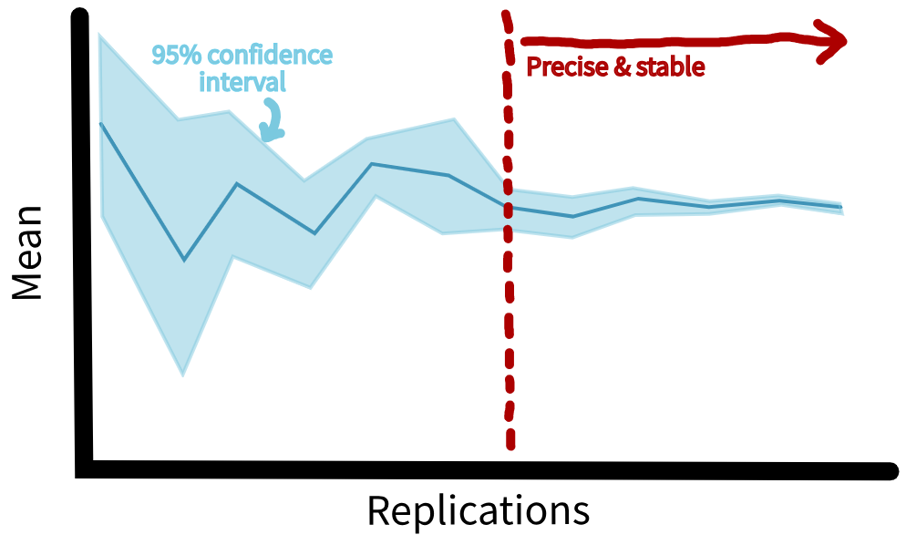
When selecting the number of replications you should repeat the analysis for all performance measures and select the highest value as your number of replications.
We’ll show two ways of implementing this: manually and automated.
Simulation code
The simulation being used is that from the Replications page.
Note
On this page, we will use a longer warm-up and run length than the short illustrative values used earlier (i.e., 30 minute warm-up, 40 minute data collection).
We are not using the previously determined warm-up length, but have simply chosen reasonably long values for this example. Very short runs, like 30/40 minutes, will be unstable and need many replications to achieve reliable outcomes.
As before, these assumptions are for demonstration only, and in later examples we will return to the shorter parameter settings for simplicity.
Manual inspection
To begin, we run our simulation model for multiple replications using our usual workflow. Here, we have set to run for 50 replications.
For this analysis, we are interested in the mean results from each replication (result["run"]).
# Run simulation for multiple replications
runner = Runner(param=Parameters(warm_up_period=10000,
                                 data_collection_period=10000,
                                 number_of_runs=50))
result = runner.run_reps()
HTML(to_html_datatable(result["run"]))| Loading ITables v2.5.2 from the internet... (need help?) |
We pass these results to the confidence_interval_method function from the sim-tools package.
The desired_precision parameter is set to 0.1, which means we are interested in identifying when the percentage deviation of the confidence interval from the mean falls below 10%. Note: This threshold is our default but relatively arbitrary. We are just using it to help us identify the point where results are stable enough.
# Define metrics to inspect
metrics = ["mean_wait_time", "mean_utilisation_tw", "mean_queue_length",
           "mean_time_in_system", "mean_patients_in_system"]

# Run the confidence interval method
confint_results = confidence_interval_method(
    replications=result["run"][metrics],
    desired_precision=0.1,
    min_rep=5,
    decimal_places=6
)
For each metric, the function returns:
- The number of replications required for deviation to fall below 10% (and must also be higher than
min_repset inconfidence_interval_method()). - A dataframe of cumulative calculations: the mean, cumulative mean, standard deviation, confidence interval bounds, and the percentage deviation of the confidence interval from the mean (displayed in the far-right column).
print(confint_results["mean_wait_time"][0])24HTML(to_html_datatable(confint_results["mean_wait_time"][1]))| Loading ITables v2.5.2 from the internet... (need help?) |
print(confint_results["mean_utilisation_tw"][0])6HTML(to_html_datatable(confint_results["mean_utilisation_tw"][1]))| Loading ITables v2.5.2 from the internet... (need help?) |
print(confint_results["mean_queue_length"][0])24HTML(to_html_datatable(confint_results["mean_queue_length"][1]))| Loading ITables v2.5.2 from the internet... (need help?) |
print(confint_results["mean_time_in_system"][0])9HTML(to_html_datatable(confint_results["mean_time_in_system"][1]))| Loading ITables v2.5.2 from the internet... (need help?) |
print(confint_results["mean_patients_in_system"][0])9HTML(to_html_datatable(confint_results["mean_patients_in_system"][1]))| Loading ITables v2.5.2 from the internet... (need help?) |
To visualise when precision is achieved and check for stability, we can use the plotly_confidence_interval_method function from sim-tools:
p = plotly_confidence_interval_method(
    n_reps=confint_results["mean_wait_time"][0],
    conf_ints=confint_results["mean_wait_time"][1],
    metric_name="Mean Wait Time")
p.update_layout(autosize=True, width=None, height=390)
p = plotly_confidence_interval_method(
n_reps=confint_results["mean_utilisation_tw"][0],
conf_ints=confint_results["mean_utilisation_tw"][1],
metric_name="Mean Utilisation")
p.update_layout(autosize=True, width=None, height=390)p = plotly_confidence_interval_method(
n_reps=confint_results["mean_queue_length"][0],
conf_ints=confint_results["mean_queue_length"][1],
metric_name="Mean Queue Length")
p.update_layout(autosize=True, width=None, height=390)p = plotly_confidence_interval_method(
n_reps=confint_results["mean_time_in_system"][0],
conf_ints=confint_results["mean_time_in_system"][1],
metric_name="Mean Time In System")
p.update_layout(autosize=True, width=None, height=390)p = plotly_confidence_interval_method(
n_reps=confint_results["mean_patients_in_system"][0],
conf_ints=confint_results["mean_patients_in_system"][1],
metric_name="Mean Patients In System")
p.update_layout(autosize=True, width=None, height=390)For this analysis, we have created two functions confidence_interval_method and plot_replication_ci.
NoteView functions
#' Use the confidence interval method to select the number of replications.
#'
#' This could be altered to use WelfordStats and ReplicationTabuliser if
#' desired, but currently is independent.
#'
#' @param param List of parameters for the model.
#' @param desired_precision Desired mean deviation from confidence interval.
#' @param metric Name of performance metric to assess.
#' @param verbose Boolean, whether to print messages about parameters.
#'
#' @importFrom rlang .data
#' @importFrom utils tail
#'
#' @return Dataframe with results from each replication.
#' @export

confidence_interval_method <- function(
  param, desired_precision, metric, verbose = TRUE
) {
  # Run model for specified number of replications
  if (isTRUE(verbose)) {
    print(param)
  }
  results <- runner(param = param)[["run_results"]]

  # Initialise list to store the results
  cumulative_list <- list()

  # For each row in the dataframe, filter to rows up to the i-th replication
  # then perform calculations
  for (i in 1L:param[["number_of_runs"]]) {

    # Filter rows up to the i-th replication
    subset_data <- results[[metric]][1L:i]

    # Get latest data point
    last_data_point <- tail(subset_data, n = 1L)

    # Calculate mean
    mean_value <- mean(subset_data)

    # Some calculations require a few observations else will error...
    if (i < 3L) {
      # When only one observation, set to NA
      stdev <- NA
      lower_ci <- NA
      upper_ci <- NA
      deviation <- NA
    } else {
      # Else, calculate standard deviation, 95% confidence interval, and
      # percentage deviation
      stdev <- stats::sd(subset_data)
      ci <- stats::t.test(subset_data)[["conf.int"]]
      lower_ci <- ci[[1L]]
      upper_ci <- ci[[2L]]
      deviation <- ((upper_ci - mean_value) / mean_value)
    }

    # Append to the cumulative list
    cumulative_list[[i]] <- data.frame(
      replications = i,
      data = last_data_point,
      cumulative_mean = mean_value,
      stdev = stdev,
      lower_ci = lower_ci,
      upper_ci = upper_ci,
      deviation = deviation
    )
  }

  # Combine the list into a single data frame
  cumulative <- do.call(rbind, cumulative_list)
  cumulative[["metric"]] <- metric

  # Get the minimum number of replications where deviation is less than target
  compare <- dplyr::filter(
    cumulative, .data[["deviation"]] <= desired_precision
  )
  if (nrow(compare) > 0L) {
    # Get minimum number
    n_reps <- compare |>
      dplyr::slice_head() |>
      dplyr::select(replications) |>
      dplyr::pull()
    message("Reached desired precision (", desired_precision, ") in ",
            n_reps, " replications.")
  } else {
    warning("Running ", param[["number_of_runs"]], " replications did not ",
            "reach desired precision (", desired_precision, ").",
            call. = FALSE)
  }
  cumulative
}
#' Generate a plot of metric and confidence intervals with increasing
#' simulation replications
#'
#' @param conf_ints A dataframe containing confidence interval statistics,
#' including cumulative mean, upper/lower bounds, and deviations. As returned
#' by ReplicationTabuliser summary_table() method.
#' @param yaxis_title Label for y axis.
#' @param file_path Path and filename to save the plot to.
#' @param min_rep The number of replications required to meet the desired
#' precision.
#'
#' @return A ggplot object if file_path is NULL; otherwise, the plot is saved
#' to file and NULL is returned invisibly.
#' @export
plot_replication_ci <- function(
conf_ints, yaxis_title, file_path = NULL, min_rep = NULL
) {
# Plot the cumulative mean and confidence interval
p <- ggplot2::ggplot(conf_ints,
ggplot2::aes(x = .data[["replications"]],
y = .data[["cumulative_mean"]])) +
ggplot2::geom_line() +
ggplot2::geom_ribbon(
ggplot2::aes(ymin = .data[["lower_ci"]], ymax = .data[["upper_ci"]]),
alpha = 0.2
)
# If specified, plot the minimum suggested number of replications
if (!is.null(min_rep)) {
p <- p +
ggplot2::geom_vline(
xintercept = min_rep, linetype = "dashed", color = "red"
)
}
# Modify labels and style
p <- p +
ggplot2::labs(x = "Replications", y = yaxis_title) +
ggplot2::theme_minimal()
# Save the plot
if (!is.null(file_path)) {
ggplot2::ggsave(filename = file_path,
width = 6.5, height = 4L, bg = "white")
} else {
p
}
}metrics <- c("mean_wait_time_doctor", "utilisation_doctor",
"mean_queue_length_doctor", "mean_time_in_system",
"mean_patients_in_system")
ci_df <- list()
for (m in metrics) {
ci_df[[m]] <- confidence_interval_method(
param = create_params(warm_up_period = 10000L,
data_collection_period = 10000L,
number_of_runs = 50L),
desired_precision = 0.1,
metric = m,
verbose = FALSE
)
}Reached desired precision (0.1) in 18 replications.Reached desired precision (0.1) in 3 replications.Reached desired precision (0.1) in 19 replications.Reached desired precision (0.1) in 3 replications.Reached desired precision (0.1) in 6 replications.ci_df[["mean_wait_time_doctor"]] |>
kable() |>
scroll_box(height = "400px")| replications | data | cumulative_mean | stdev | lower_ci | upper_ci | deviation | metric |
|---|---|---|---|---|---|---|---|
| 1 | 5.667672 | 5.667672 | NA | NA | NA | NA | mean_wait_time_doctor |
| 2 | 5.328368 | 5.498020 | NA | NA | NA | NA | mean_wait_time_doctor |
| 3 | 4.934004 | 5.310015 | 0.3671783 | 4.397893 | 6.222136 | 0.1717738 | mean_wait_time_doctor |
| 4 | 3.671831 | 4.900469 | 0.8722335 | 3.512551 | 6.288387 | 0.2832215 | mean_wait_time_doctor |
| 5 | 3.412813 | 4.602938 | 1.0065869 | 3.353095 | 5.852780 | 0.2715315 | mean_wait_time_doctor |
| 6 | 5.059963 | 4.679109 | 0.9194487 | 3.714206 | 5.644011 | 0.2062150 | mean_wait_time_doctor |
| 7 | 4.842750 | 4.702486 | 0.8416138 | 3.924123 | 5.480849 | 0.1655216 | mean_wait_time_doctor |
| 8 | 4.862139 | 4.722443 | 0.7812248 | 4.069322 | 5.375563 | 0.1383014 | mean_wait_time_doctor |
| 9 | 4.667285 | 4.716314 | 0.7310001 | 4.154418 | 5.278210 | 0.1191389 | mean_wait_time_doctor |
| 10 | 6.072426 | 4.851925 | 0.8117215 | 4.271255 | 5.432596 | 0.1196784 | mean_wait_time_doctor |
| 11 | 4.269149 | 4.798946 | 0.7898594 | 4.268311 | 5.329580 | 0.1105732 | mean_wait_time_doctor |
| 12 | 3.412673 | 4.683423 | 0.8528233 | 4.141565 | 5.225281 | 0.1156970 | mean_wait_time_doctor |
| 13 | 4.891019 | 4.699392 | 0.8185437 | 4.204751 | 5.194033 | 0.1052564 | mean_wait_time_doctor |
| 14 | 3.492198 | 4.613164 | 0.8500401 | 4.122365 | 5.103962 | 0.1063909 | mean_wait_time_doctor |
| 15 | 3.890397 | 4.564979 | 0.8401085 | 4.099743 | 5.030216 | 0.1019143 | mean_wait_time_doctor |
| 16 | 2.990553 | 4.466578 | 0.9020290 | 3.985920 | 4.947235 | 0.1076120 | mean_wait_time_doctor |
| 17 | 5.359595 | 4.519108 | 0.8998408 | 4.056452 | 4.981763 | 0.1023776 | mean_wait_time_doctor |
| 18 | 3.888761 | 4.484089 | 0.8855267 | 4.043727 | 4.924451 | 0.0982055 | mean_wait_time_doctor |
| 19 | 3.689211 | 4.442253 | 0.8796859 | 4.018258 | 4.866248 | 0.0954459 | mean_wait_time_doctor |
| 20 | 4.288418 | 4.434561 | 0.8569141 | 4.033513 | 4.835610 | 0.0904369 | mean_wait_time_doctor |
| 21 | 4.359718 | 4.430997 | 0.8353762 | 4.050739 | 4.811256 | 0.0858179 | mean_wait_time_doctor |
| 22 | 3.882755 | 4.406077 | 0.8235803 | 4.040922 | 4.771232 | 0.0828753 | mean_wait_time_doctor |
| 23 | 4.639772 | 4.416238 | 0.8061191 | 4.067646 | 4.764830 | 0.0789342 | mean_wait_time_doctor |
| 24 | 3.956291 | 4.397074 | 0.7939705 | 4.061809 | 4.732338 | 0.0762472 | mean_wait_time_doctor |
| 25 | 4.254914 | 4.391387 | 0.7777733 | 4.070338 | 4.712436 | 0.0731088 | mean_wait_time_doctor |
| 26 | 4.701406 | 4.403311 | 0.7644807 | 4.094531 | 4.712091 | 0.0701246 | mean_wait_time_doctor |
| 27 | 5.532829 | 4.445145 | 0.7805157 | 4.136383 | 4.753907 | 0.0694604 | mean_wait_time_doctor |
| 28 | 5.432689 | 4.480414 | 0.7883348 | 4.174730 | 4.786099 | 0.0682268 | mean_wait_time_doctor |
| 29 | 4.290552 | 4.473867 | 0.7749318 | 4.179099 | 4.768636 | 0.0658867 | mean_wait_time_doctor |
| 30 | 3.302238 | 4.434813 | 0.7909292 | 4.139475 | 4.730151 | 0.0665953 | mean_wait_time_doctor |
| 31 | 3.791986 | 4.414077 | 0.7861594 | 4.125711 | 4.702442 | 0.0653286 | mean_wait_time_doctor |
| 32 | 3.405390 | 4.382555 | 0.7936654 | 4.096408 | 4.668702 | 0.0652923 | mean_wait_time_doctor |
| 33 | 3.714474 | 4.362310 | 0.7897756 | 4.082268 | 4.642353 | 0.0641959 | mean_wait_time_doctor |
| 34 | 4.399654 | 4.363409 | 0.7777436 | 4.092041 | 4.634776 | 0.0621917 | mean_wait_time_doctor |
| 35 | 5.318725 | 4.390703 | 0.7830515 | 4.121716 | 4.659691 | 0.0612630 | mean_wait_time_doctor |
| 36 | 6.269489 | 4.442892 | 0.8328874 | 4.161083 | 4.724700 | 0.0634291 | mean_wait_time_doctor |
| 37 | 6.217519 | 4.490855 | 0.8715206 | 4.200275 | 4.781434 | 0.0647047 | mean_wait_time_doctor |
| 38 | 4.550575 | 4.492426 | 0.8597173 | 4.209844 | 4.775008 | 0.0629019 | mean_wait_time_doctor |
| 39 | 4.366934 | 4.489209 | 0.8485677 | 4.214135 | 4.764283 | 0.0612745 | mean_wait_time_doctor |
| 40 | 3.594789 | 4.466848 | 0.8494726 | 4.195174 | 4.738523 | 0.0608202 | mean_wait_time_doctor |
| 41 | 4.340154 | 4.463758 | 0.8390203 | 4.198931 | 4.728586 | 0.0593284 | mean_wait_time_doctor |
| 42 | 5.209670 | 4.481518 | 0.8366795 | 4.220790 | 4.742246 | 0.0581784 | mean_wait_time_doctor |
| 43 | 3.739431 | 4.464260 | 0.8343692 | 4.207479 | 4.721041 | 0.0575193 | mean_wait_time_doctor |
| 44 | 4.902840 | 4.474228 | 0.8272567 | 4.222719 | 4.725737 | 0.0562128 | mean_wait_time_doctor |
| 45 | 3.445952 | 4.451377 | 0.8320438 | 4.201403 | 4.701351 | 0.0561565 | mean_wait_time_doctor |
| 46 | 3.791042 | 4.437022 | 0.8284876 | 4.190992 | 4.683052 | 0.0554495 | mean_wait_time_doctor |
| 47 | 4.572846 | 4.439912 | 0.8196723 | 4.199247 | 4.680577 | 0.0542049 | mean_wait_time_doctor |
| 48 | 5.344848 | 4.458765 | 0.8213576 | 4.220267 | 4.697262 | 0.0534896 | mean_wait_time_doctor |
| 49 | 3.817683 | 4.445681 | 0.8179004 | 4.210753 | 4.680610 | 0.0528442 | mean_wait_time_doctor |
| 50 | 4.078986 | 4.438347 | 0.8111708 | 4.207815 | 4.668880 | 0.0519410 | mean_wait_time_doctor |
plot_replication_ci(
  conf_ints = ci_df[["mean_wait_time_doctor"]],
  yaxis_title = "Mean wait time",
  min_rep = 5L
)
Warning: Removed 2 rows containing missing values or values outside the scale range
(`geom_ribbon()`).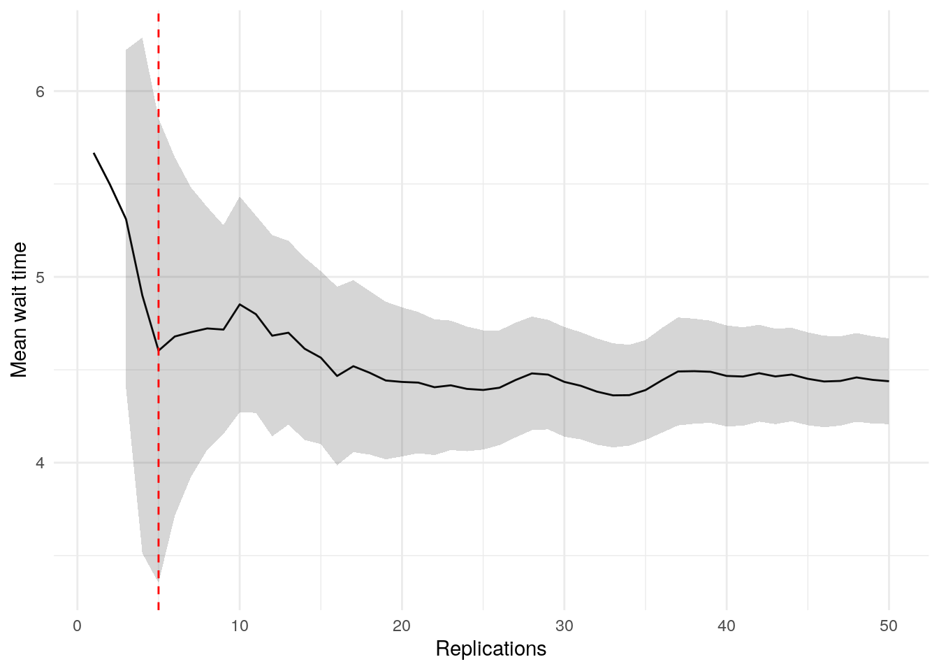
ci_df[["utilisation_doctor"]] |>
  kable() |>
scroll_box(height = "400px")| replications | data | cumulative_mean | stdev | lower_ci | upper_ci | deviation | metric |
|---|---|---|---|---|---|---|---|
| 1 | 0.6832362 | 0.6832362 | NA | NA | NA | NA | utilisation_doctor |
| 2 | 0.7014341 | 0.6923351 | NA | NA | NA | NA | utilisation_doctor |
| 3 | 0.6503975 | 0.6783559 | 0.0258659 | 0.6141014 | 0.7426104 | 0.0947210 | utilisation_doctor |
| 4 | 0.6437990 | 0.6697167 | 0.0272869 | 0.6262971 | 0.7131363 | 0.0648327 | utilisation_doctor |
| 5 | 0.6789189 | 0.6715571 | 0.0239868 | 0.6417735 | 0.7013407 | 0.0443500 | utilisation_doctor |
| 6 | 0.6713653 | 0.6715251 | 0.0214546 | 0.6490099 | 0.6940404 | 0.0335285 | utilisation_doctor |
| 7 | 0.6775094 | 0.6723800 | 0.0197155 | 0.6541463 | 0.6906138 | 0.0271182 | utilisation_doctor |
| 8 | 0.6528520 | 0.6699390 | 0.0195151 | 0.6536240 | 0.6862541 | 0.0243530 | utilisation_doctor |
| 9 | 0.6541008 | 0.6681792 | 0.0190028 | 0.6535724 | 0.6827861 | 0.0218607 | utilisation_doctor |
| 10 | 0.6893232 | 0.6702936 | 0.0191230 | 0.6566138 | 0.6839734 | 0.0204087 | utilisation_doctor |
| 11 | 0.6477562 | 0.6682448 | 0.0193726 | 0.6552301 | 0.6812594 | 0.0194759 | utilisation_doctor |
| 12 | 0.6335263 | 0.6653516 | 0.0210149 | 0.6519993 | 0.6787038 | 0.0200680 | utilisation_doctor |
| 13 | 0.6503795 | 0.6641999 | 0.0205443 | 0.6517851 | 0.6766147 | 0.0186913 | utilisation_doctor |
| 14 | 0.6284034 | 0.6616430 | 0.0219347 | 0.6489783 | 0.6743077 | 0.0191413 | utilisation_doctor |
| 15 | 0.6647776 | 0.6618519 | 0.0211523 | 0.6501382 | 0.6735657 | 0.0176984 | utilisation_doctor |
| 16 | 0.6282434 | 0.6597514 | 0.0220949 | 0.6479779 | 0.6715250 | 0.0178454 | utilisation_doctor |
| 17 | 0.6814358 | 0.6610270 | 0.0220303 | 0.6497000 | 0.6723539 | 0.0171354 | utilisation_doctor |
| 18 | 0.6703249 | 0.6615435 | 0.0214846 | 0.6508595 | 0.6722276 | 0.0161502 | utilisation_doctor |
| 19 | 0.6278075 | 0.6597679 | 0.0222676 | 0.6490353 | 0.6705006 | 0.0162673 | utilisation_doctor |
| 20 | 0.6750253 | 0.6605308 | 0.0219405 | 0.6502623 | 0.6707993 | 0.0155458 | utilisation_doctor |
| 21 | 0.6663518 | 0.6608080 | 0.0214227 | 0.6510565 | 0.6705595 | 0.0147569 | utilisation_doctor |
| 22 | 0.6746140 | 0.6614355 | 0.0211126 | 0.6520747 | 0.6707963 | 0.0141522 | utilisation_doctor |
| 23 | 0.6796506 | 0.6622275 | 0.0209739 | 0.6531577 | 0.6712973 | 0.0136959 | utilisation_doctor |
| 24 | 0.6635614 | 0.6622831 | 0.0205147 | 0.6536205 | 0.6709457 | 0.0130799 | utilisation_doctor |
| 25 | 0.6439847 | 0.6615511 | 0.0204135 | 0.6531249 | 0.6699774 | 0.0127372 | utilisation_doctor |
| 26 | 0.6548798 | 0.6612946 | 0.0200438 | 0.6531987 | 0.6693904 | 0.0122425 | utilisation_doctor |
| 27 | 0.6608308 | 0.6612774 | 0.0196548 | 0.6535022 | 0.6690526 | 0.0117578 | utilisation_doctor |
| 28 | 0.6865314 | 0.6621793 | 0.0198691 | 0.6544749 | 0.6698837 | 0.0116349 | utilisation_doctor |
| 29 | 0.6431757 | 0.6615240 | 0.0198276 | 0.6539820 | 0.6690660 | 0.0114010 | utilisation_doctor |
| 30 | 0.6628206 | 0.6615672 | 0.0194842 | 0.6542917 | 0.6688427 | 0.0109974 | utilisation_doctor |
| 31 | 0.6217329 | 0.6602823 | 0.0204491 | 0.6527815 | 0.6677830 | 0.0113600 | utilisation_doctor |
| 32 | 0.6519350 | 0.6600214 | 0.0201706 | 0.6527491 | 0.6672937 | 0.0110182 | utilisation_doctor |
| 33 | 0.6551604 | 0.6598741 | 0.0198710 | 0.6528282 | 0.6669200 | 0.0106777 | utilisation_doctor |
| 34 | 0.6686245 | 0.6601315 | 0.0196250 | 0.6532840 | 0.6669790 | 0.0103729 | utilisation_doctor |
| 35 | 0.6902273 | 0.6609913 | 0.0199923 | 0.6541237 | 0.6678590 | 0.0103899 | utilisation_doctor |
| 36 | 0.6739451 | 0.6613512 | 0.0198226 | 0.6546442 | 0.6680582 | 0.0101414 | utilisation_doctor |
| 37 | 0.6806258 | 0.6618721 | 0.0198005 | 0.6552703 | 0.6684739 | 0.0099745 | utilisation_doctor |
| 38 | 0.6504647 | 0.6615719 | 0.0196186 | 0.6551234 | 0.6680204 | 0.0097472 | utilisation_doctor |
| 39 | 0.6712074 | 0.6618190 | 0.0194201 | 0.6555237 | 0.6681142 | 0.0095121 | utilisation_doctor |
| 40 | 0.6725828 | 0.6620881 | 0.0192449 | 0.6559333 | 0.6682429 | 0.0092961 | utilisation_doctor |
| 41 | 0.6568020 | 0.6619591 | 0.0190208 | 0.6559555 | 0.6679628 | 0.0090696 | utilisation_doctor |
| 42 | 0.6883579 | 0.6625877 | 0.0192239 | 0.6565971 | 0.6685783 | 0.0090412 | utilisation_doctor |
| 43 | 0.6484279 | 0.6622584 | 0.0191160 | 0.6563754 | 0.6681414 | 0.0088833 | utilisation_doctor |
| 44 | 0.6631406 | 0.6622784 | 0.0188929 | 0.6565345 | 0.6680224 | 0.0086730 | utilisation_doctor |
| 45 | 0.6412090 | 0.6618102 | 0.0189392 | 0.6561203 | 0.6675002 | 0.0085976 | utilisation_doctor |
| 46 | 0.6604320 | 0.6617803 | 0.0187287 | 0.6562185 | 0.6673420 | 0.0084042 | utilisation_doctor |
| 47 | 0.6436991 | 0.6613956 | 0.0187108 | 0.6559019 | 0.6668893 | 0.0083062 | utilisation_doctor |
| 48 | 0.6934467 | 0.6620633 | 0.0190800 | 0.6565230 | 0.6676036 | 0.0083682 | utilisation_doctor |
| 49 | 0.6702343 | 0.6622300 | 0.0189163 | 0.6567967 | 0.6676634 | 0.0082047 | utilisation_doctor |
| 50 | 0.6737071 | 0.6624596 | 0.0187925 | 0.6571188 | 0.6678004 | 0.0080620 | utilisation_doctor |
plot_replication_ci(
  conf_ints = ci_df[["utilisation_doctor"]],
  yaxis_title = "Utilisation",
  min_rep = 5L
)
Warning: Removed 2 rows containing missing values or values outside the scale range
(`geom_ribbon()`).
ci_df[["mean_queue_length_doctor"]] |>
  kable() |>
scroll_box(height = "400px")| replications | data | cumulative_mean | stdev | lower_ci | upper_ci | deviation | metric |
|---|---|---|---|---|---|---|---|
| 1 | 1.2047321 | 1.2047321 | NA | NA | NA | NA | mean_queue_length_doctor |
| 2 | 1.0585763 | 1.1316542 | NA | NA | NA | NA | mean_queue_length_doctor |
| 3 | 1.0061322 | 1.0898135 | 0.1029189 | 0.8341487 | 1.3454783 | 0.2345950 | mean_queue_length_doctor |
| 4 | 0.7220796 | 0.9978800 | 0.2021598 | 0.6761987 | 1.3195614 | 0.3223648 | mean_queue_length_doctor |
| 5 | 0.7147191 | 0.9412479 | 0.2160728 | 0.6729580 | 1.2095377 | 0.2850363 | mean_queue_length_doctor |
| 6 | 0.9998528 | 0.9510153 | 0.1947367 | 0.7466517 | 1.1553790 | 0.2148900 | mean_queue_length_doctor |
| 7 | 0.9630582 | 0.9527358 | 0.1778278 | 0.7882725 | 1.1171990 | 0.1726221 | mean_queue_length_doctor |
| 8 | 0.9401393 | 0.9511612 | 0.1646967 | 0.8134713 | 1.0888511 | 0.1447598 | mean_queue_length_doctor |
| 9 | 0.9319599 | 0.9490277 | 0.1541926 | 0.8305048 | 1.0675506 | 0.1248888 | mean_queue_length_doctor |
| 10 | 1.2095963 | 0.9750846 | 0.1671025 | 0.8555466 | 1.0946225 | 0.1225924 | mean_queue_length_doctor |
| 11 | 0.8724811 | 0.9657570 | 0.1615177 | 0.8572479 | 1.0742660 | 0.1123565 | mean_queue_length_doctor |
| 12 | 0.6465119 | 0.9391532 | 0.1794699 | 0.8251235 | 1.0531830 | 0.1214176 | mean_queue_length_doctor |
| 13 | 0.9578633 | 0.9405925 | 0.1719077 | 0.8367097 | 1.0444752 | 0.1104440 | mean_queue_length_doctor |
| 14 | 0.7166333 | 0.9245954 | 0.1756750 | 0.8231637 | 1.0260271 | 0.1097039 | mean_queue_length_doctor |
| 15 | 0.7937702 | 0.9158737 | 0.1726219 | 0.8202789 | 1.0114685 | 0.1043755 | mean_queue_length_doctor |
| 16 | 0.5950870 | 0.8958245 | 0.1850493 | 0.7972187 | 0.9944304 | 0.1100727 | mean_queue_length_doctor |
| 17 | 1.0952642 | 0.9075563 | 0.1855878 | 0.8121358 | 1.0029767 | 0.1051400 | mean_queue_length_doctor |
| 18 | 0.7925600 | 0.9011676 | 0.1820754 | 0.8106236 | 0.9917116 | 0.1004741 | mean_queue_length_doctor |
| 19 | 0.7424607 | 0.8928146 | 0.1806527 | 0.8057428 | 0.9798864 | 0.0975251 | mean_queue_length_doctor |
| 20 | 0.8539327 | 0.8908705 | 0.1760492 | 0.8084769 | 0.9732641 | 0.0924866 | mean_queue_length_doctor |
| 21 | 0.8341843 | 0.8881712 | 0.1720368 | 0.8098609 | 0.9664814 | 0.0881702 | mean_queue_length_doctor |
| 22 | 0.7866429 | 0.8835562 | 0.1692804 | 0.8085015 | 0.9586110 | 0.0849462 | mean_queue_length_doctor |
| 23 | 0.9277437 | 0.8854774 | 0.1656448 | 0.8138472 | 0.9571076 | 0.0808944 | mean_queue_length_doctor |
| 24 | 0.7972331 | 0.8818006 | 0.1630022 | 0.8129708 | 0.9506304 | 0.0780559 | mean_queue_length_doctor |
| 25 | 0.8530547 | 0.8806507 | 0.1596737 | 0.8147407 | 0.9465608 | 0.0748424 | mean_queue_length_doctor |
| 26 | 0.9224187 | 0.8822572 | 0.1566619 | 0.8189801 | 0.9455343 | 0.0717219 | mean_queue_length_doctor |
| 27 | 1.1294072 | 0.8914109 | 0.1608146 | 0.8277948 | 0.9550270 | 0.0713657 | mean_queue_length_doctor |
| 28 | 1.0772452 | 0.8980478 | 0.1616690 | 0.8353591 | 0.9607366 | 0.0698055 | mean_queue_length_doctor |
| 29 | 0.8531167 | 0.8964985 | 0.1589749 | 0.8360277 | 0.9569693 | 0.0674522 | mean_queue_length_doctor |
| 30 | 0.6787016 | 0.8892386 | 0.1611916 | 0.8290487 | 0.9494285 | 0.0676870 | mean_queue_length_doctor |
| 31 | 0.7243055 | 0.8839182 | 0.1612270 | 0.8247796 | 0.9430567 | 0.0669050 | mean_queue_length_doctor |
| 32 | 0.6910776 | 0.8778919 | 0.1622274 | 0.8194027 | 0.9363811 | 0.0666246 | mean_queue_length_doctor |
| 33 | 0.7121484 | 0.8728694 | 0.1622583 | 0.8153351 | 0.9304037 | 0.0659140 | mean_queue_length_doctor |
| 34 | 0.9340725 | 0.8746695 | 0.1601253 | 0.8187991 | 0.9305398 | 0.0638760 | mean_queue_length_doctor |
| 35 | 1.1099986 | 0.8813932 | 0.1626908 | 0.8255069 | 0.9372794 | 0.0634067 | mean_queue_length_doctor |
| 36 | 1.2898175 | 0.8927383 | 0.1742001 | 0.8337975 | 0.9516791 | 0.0660225 | mean_queue_length_doctor |
| 37 | 1.2600902 | 0.9026667 | 0.1820713 | 0.8419611 | 0.9633723 | 0.0672514 | mean_queue_length_doctor |
| 38 | 0.9610278 | 0.9042025 | 0.1798434 | 0.8450895 | 0.9633156 | 0.0653759 | mean_queue_length_doctor |
| 39 | 0.8588293 | 0.9030391 | 0.1776099 | 0.8454646 | 0.9606136 | 0.0637564 | mean_queue_length_doctor |
| 40 | 0.7175814 | 0.8984027 | 0.1777535 | 0.8415544 | 0.9552510 | 0.0632771 | mean_queue_length_doctor |
| 41 | 0.8762122 | 0.8978614 | 0.1755517 | 0.8424505 | 0.9532724 | 0.0617144 | mean_queue_length_doctor |
| 42 | 1.0504412 | 0.9014943 | 0.1749887 | 0.8469640 | 0.9560246 | 0.0604888 | mean_queue_length_doctor |
| 43 | 0.7479977 | 0.8979246 | 0.1744703 | 0.8442306 | 0.9516186 | 0.0597979 | mean_queue_length_doctor |
| 44 | 1.0019122 | 0.9002880 | 0.1731408 | 0.8476483 | 0.9529276 | 0.0584698 | mean_queue_length_doctor |
| 45 | 0.6953367 | 0.8957335 | 0.1738674 | 0.8434979 | 0.9479690 | 0.0583160 | mean_queue_length_doctor |
| 46 | 0.7645500 | 0.8928817 | 0.1730093 | 0.8415043 | 0.9442591 | 0.0575411 | mean_queue_length_doctor |
| 47 | 0.9318572 | 0.8937109 | 0.1712129 | 0.8434410 | 0.9439809 | 0.0562486 | mean_queue_length_doctor |
| 48 | 1.0725052 | 0.8974358 | 0.1713363 | 0.8476849 | 0.9471867 | 0.0554367 | mean_queue_length_doctor |
| 49 | 0.8105346 | 0.8956623 | 0.1699961 | 0.8468338 | 0.9444909 | 0.0545167 | mean_queue_length_doctor |
| 50 | 0.8308819 | 0.8943667 | 0.1685017 | 0.8464791 | 0.9422544 | 0.0535436 | mean_queue_length_doctor |
plot_replication_ci(
  conf_ints = ci_df[["mean_queue_length_doctor"]],
  yaxis_title = "Mean queue length",
  min_rep = 5L
)
Warning: Removed 2 rows containing missing values or values outside the scale range
(`geom_ribbon()`).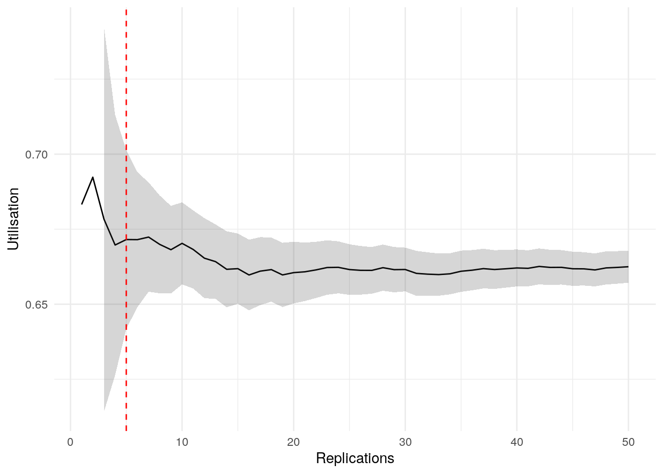
ci_df[["mean_time_in_system"]] |>
  kable() |>
scroll_box(height = "400px")| replications | data | cumulative_mean | stdev | lower_ci | upper_ci | deviation | metric |
|---|---|---|---|---|---|---|---|
| 1 | 15.58670 | 15.58670 | NA | NA | NA | NA | mean_time_in_system |
| 2 | 15.64705 | 15.61688 | NA | NA | NA | NA | mean_time_in_system |
| 3 | 14.80302 | 15.34559 | 0.4708495 | 14.17594 | 16.51525 | 0.0762209 | mean_time_in_system |
| 4 | 13.42023 | 14.86425 | 1.0366078 | 13.21478 | 16.51372 | 0.1109692 | mean_time_in_system |
| 5 | 13.41904 | 14.57521 | 1.1061844 | 13.20170 | 15.94872 | 0.0942360 | mean_time_in_system |
| 6 | 14.99688 | 14.64549 | 1.0042656 | 13.59157 | 15.69940 | 0.0719616 | mean_time_in_system |
| 7 | 15.06660 | 14.70564 | 0.9304792 | 13.84509 | 15.56619 | 0.0585183 | mean_time_in_system |
| 8 | 14.92535 | 14.73311 | 0.8649513 | 14.00999 | 15.45622 | 0.0490811 | mean_time_in_system |
| 9 | 14.23345 | 14.67759 | 0.8260523 | 14.04263 | 15.31255 | 0.0432605 | mean_time_in_system |
| 10 | 16.53909 | 14.86374 | 0.9762495 | 14.16537 | 15.56211 | 0.0469846 | mean_time_in_system |
| 11 | 14.02954 | 14.78790 | 0.9596977 | 14.14317 | 15.43264 | 0.0435987 | mean_time_in_system |
| 12 | 13.17471 | 14.65347 | 1.0267213 | 14.00112 | 15.30582 | 0.0445183 | mean_time_in_system |
| 13 | 14.92982 | 14.67473 | 0.9859944 | 14.07890 | 15.27056 | 0.0406025 | mean_time_in_system |
| 14 | 12.87660 | 14.54629 | 1.0622377 | 13.93297 | 15.15961 | 0.0421632 | mean_time_in_system |
| 15 | 13.82593 | 14.49827 | 1.0403592 | 13.92214 | 15.07440 | 0.0397380 | mean_time_in_system |
| 16 | 12.73663 | 14.38816 | 1.0973382 | 13.80343 | 14.97290 | 0.0406397 | mean_time_in_system |
| 17 | 15.39315 | 14.44728 | 1.0900934 | 13.88681 | 15.00776 | 0.0387944 | mean_time_in_system |
| 18 | 13.73073 | 14.40747 | 1.0709475 | 13.87490 | 14.94004 | 0.0369648 | mean_time_in_system |
| 19 | 13.36509 | 14.35261 | 1.0678943 | 13.83790 | 14.86732 | 0.0358617 | mean_time_in_system |
| 20 | 14.33452 | 14.35171 | 1.0394199 | 13.86524 | 14.83817 | 0.0338959 | mean_time_in_system |
| 21 | 14.52219 | 14.35982 | 1.0137840 | 13.89836 | 14.82129 | 0.0321361 | mean_time_in_system |
| 22 | 13.99784 | 14.34337 | 0.9923574 | 13.90338 | 14.78336 | 0.0306753 | mean_time_in_system |
| 23 | 14.60215 | 14.35462 | 0.9710418 | 13.93471 | 14.77453 | 0.0292526 | mean_time_in_system |
| 24 | 13.96176 | 14.33825 | 0.9530773 | 13.93580 | 14.74070 | 0.0280682 | mean_time_in_system |
| 25 | 13.95520 | 14.32293 | 0.9361503 | 13.93651 | 14.70935 | 0.0269794 | mean_time_in_system |
| 26 | 14.74119 | 14.33902 | 0.9208968 | 13.96706 | 14.71098 | 0.0259403 | mean_time_in_system |
| 27 | 15.33368 | 14.37586 | 0.9230796 | 14.01070 | 14.74101 | 0.0254008 | mean_time_in_system |
| 28 | 15.72428 | 14.42401 | 0.9409861 | 14.05914 | 14.78889 | 0.0252964 | mean_time_in_system |
| 29 | 14.09975 | 14.41283 | 0.9259899 | 14.06061 | 14.76506 | 0.0244385 | mean_time_in_system |
| 30 | 12.81237 | 14.35948 | 0.9556530 | 14.00264 | 14.71633 | 0.0248509 | mean_time_in_system |
| 31 | 13.79822 | 14.34138 | 0.9449825 | 13.99476 | 14.68800 | 0.0241694 | mean_time_in_system |
| 32 | 13.06655 | 14.30154 | 0.9565421 | 13.95667 | 14.64641 | 0.0241142 | mean_time_in_system |
| 33 | 13.54228 | 14.27853 | 0.9507098 | 13.94143 | 14.61564 | 0.0236094 | mean_time_in_system |
| 34 | 14.06356 | 14.27221 | 0.9369199 | 13.94530 | 14.59912 | 0.0229051 | mean_time_in_system |
| 35 | 15.32178 | 14.30220 | 0.9399334 | 13.97932 | 14.62508 | 0.0225754 | mean_time_in_system |
| 36 | 16.33737 | 14.35873 | 0.9865529 | 14.02493 | 14.69253 | 0.0232473 | mean_time_in_system |
| 37 | 16.33898 | 14.41225 | 1.0257850 | 14.07024 | 14.75426 | 0.0237308 | mean_time_in_system |
| 38 | 14.24194 | 14.40777 | 1.0122052 | 14.07507 | 14.74047 | 0.0230920 | mean_time_in_system |
| 39 | 14.38384 | 14.40715 | 0.9988053 | 14.08338 | 14.73093 | 0.0224732 | mean_time_in_system |
| 40 | 13.33151 | 14.38026 | 1.0004786 | 14.06030 | 14.70023 | 0.0222505 | mean_time_in_system |
| 41 | 14.17813 | 14.37533 | 0.9883977 | 14.06336 | 14.68731 | 0.0217022 | mean_time_in_system |
| 42 | 15.37684 | 14.39918 | 0.9884250 | 14.09116 | 14.70719 | 0.0213911 | mean_time_in_system |
| 43 | 13.58958 | 14.38035 | 0.9843604 | 14.07741 | 14.68329 | 0.0210663 | mean_time_in_system |
| 44 | 14.75626 | 14.38889 | 0.9744962 | 14.09262 | 14.68517 | 0.0205905 | mean_time_in_system |
| 45 | 13.11879 | 14.36067 | 0.9817882 | 14.06571 | 14.65563 | 0.0205396 | mean_time_in_system |
| 46 | 13.63696 | 14.34494 | 0.9766647 | 14.05490 | 14.63497 | 0.0202185 | mean_time_in_system |
| 47 | 14.18810 | 14.34160 | 0.9662613 | 14.05790 | 14.62531 | 0.0197820 | mean_time_in_system |
| 48 | 15.78832 | 14.37174 | 0.9784682 | 14.08762 | 14.65586 | 0.0197692 | mean_time_in_system |
| 49 | 13.49178 | 14.35378 | 0.9763488 | 14.07334 | 14.63422 | 0.0195377 | mean_time_in_system |
| 50 | 13.85929 | 14.34389 | 0.9688618 | 14.06854 | 14.61924 | 0.0191961 | mean_time_in_system |
plot_replication_ci(
  conf_ints = ci_df[["mean_time_in_system"]],
  yaxis_title = "Mean time in system",
  min_rep = 5L
)
Warning: Removed 2 rows containing missing values or values outside the scale range
(`geom_ribbon()`).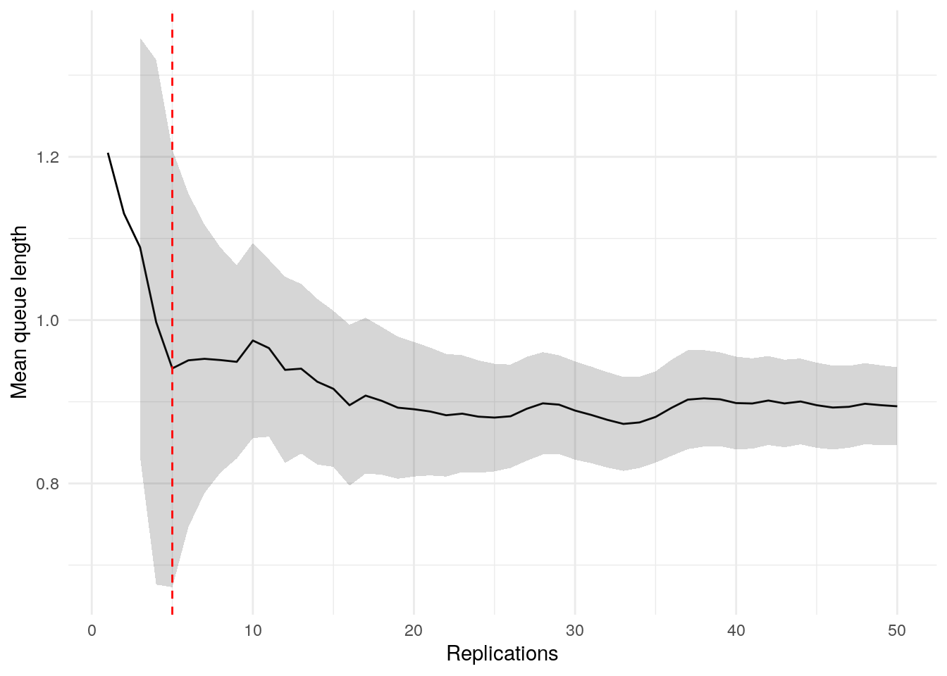
ci_df[["mean_patients_in_system"]] |>
  kable() |>
scroll_box(height = "400px")| replications | data | cumulative_mean | stdev | lower_ci | upper_ci | deviation | metric |
|---|---|---|---|---|---|---|---|
| 1 | 3.220799 | 3.220799 | NA | NA | NA | NA | mean_patients_in_system |
| 2 | 3.200296 | 3.210548 | NA | NA | NA | NA | mean_patients_in_system |
| 3 | 2.910529 | 3.110542 | 0.1735187 | 2.679497 | 3.541586 | 0.1385753 | mean_patients_in_system |
| 4 | 2.658131 | 2.997439 | 0.2669107 | 2.572724 | 3.422153 | 0.1416925 | mean_patients_in_system |
| 5 | 2.727798 | 2.943511 | 0.2607148 | 2.619791 | 3.267231 | 0.1099776 | mean_patients_in_system |
| 6 | 3.039950 | 2.959584 | 0.2364907 | 2.711402 | 3.207766 | 0.0838570 | mean_patients_in_system |
| 7 | 2.992402 | 2.964272 | 0.2162415 | 2.764282 | 3.164262 | 0.0674668 | mean_patients_in_system |
| 8 | 2.906402 | 2.957038 | 0.2012436 | 2.788795 | 3.125282 | 0.0568961 | mean_patients_in_system |
| 9 | 2.914509 | 2.952313 | 0.1887791 | 2.807205 | 3.097421 | 0.0491508 | mean_patients_in_system |
| 10 | 3.267347 | 2.983816 | 0.2039668 | 2.837907 | 3.129726 | 0.0489002 | mean_patients_in_system |
| 11 | 2.794186 | 2.966577 | 0.2017704 | 2.831026 | 3.102128 | 0.0456928 | mean_patients_in_system |
| 12 | 2.564186 | 2.933045 | 0.2247298 | 2.790258 | 3.075831 | 0.0486820 | mean_patients_in_system |
| 13 | 2.891613 | 2.929858 | 0.2154690 | 2.799651 | 3.060064 | 0.0444413 | mean_patients_in_system |
| 14 | 2.583487 | 2.905117 | 0.2267710 | 2.774183 | 3.036050 | 0.0450700 | mean_patients_in_system |
| 15 | 2.774866 | 2.896434 | 0.2210947 | 2.773995 | 3.018872 | 0.0422721 | mean_patients_in_system |
| 16 | 2.467407 | 2.869619 | 0.2390146 | 2.742257 | 2.996981 | 0.0443829 | mean_patients_in_system |
| 17 | 3.140526 | 2.885555 | 0.2405714 | 2.761865 | 3.009245 | 0.0428654 | mean_patients_in_system |
| 18 | 2.794623 | 2.880503 | 0.2343706 | 2.763953 | 2.997053 | 0.0404616 | mean_patients_in_system |
| 19 | 2.600749 | 2.865779 | 0.2366368 | 2.751724 | 2.979835 | 0.0397991 | mean_patients_in_system |
| 20 | 2.888899 | 2.866935 | 0.2303834 | 2.759113 | 2.974758 | 0.0376091 | mean_patients_in_system |
| 21 | 2.855192 | 2.866376 | 0.2245646 | 2.764156 | 2.968597 | 0.0356620 | mean_patients_in_system |
| 22 | 2.798657 | 2.863298 | 0.2196276 | 2.765921 | 2.960675 | 0.0340088 | mean_patients_in_system |
| 23 | 2.987137 | 2.868682 | 0.2161262 | 2.775222 | 2.962142 | 0.0325794 | mean_patients_in_system |
| 24 | 2.777398 | 2.864879 | 0.2121953 | 2.775276 | 2.954481 | 0.0312761 | mean_patients_in_system |
| 25 | 2.776448 | 2.861341 | 0.2084790 | 2.775286 | 2.947397 | 0.0300754 | mean_patients_in_system |
| 26 | 2.888231 | 2.862376 | 0.2043350 | 2.779843 | 2.944908 | 0.0288336 | mean_patients_in_system |
| 27 | 3.100114 | 2.871181 | 0.2055243 | 2.789878 | 2.952484 | 0.0283168 | mean_patients_in_system |
| 28 | 3.144160 | 2.880930 | 0.2081757 | 2.800208 | 2.961652 | 0.0280195 | mean_patients_in_system |
| 29 | 2.774958 | 2.877276 | 0.2053694 | 2.799158 | 2.955394 | 0.0271501 | mean_patients_in_system |
| 30 | 2.682587 | 2.870786 | 0.2049041 | 2.794274 | 2.947299 | 0.0266521 | mean_patients_in_system |
| 31 | 2.574375 | 2.861225 | 0.2083755 | 2.784792 | 2.937657 | 0.0267133 | mean_patients_in_system |
| 32 | 2.646656 | 2.854519 | 0.2084669 | 2.779359 | 2.929680 | 0.0263303 | mean_patients_in_system |
| 33 | 2.708765 | 2.850103 | 0.2067465 | 2.776794 | 2.923412 | 0.0257216 | mean_patients_in_system |
| 34 | 2.921153 | 2.852192 | 0.2039542 | 2.781029 | 2.923355 | 0.0249503 | mean_patients_in_system |
| 35 | 3.168527 | 2.861230 | 0.2079253 | 2.789806 | 2.932655 | 0.0249630 | mean_patients_in_system |
| 36 | 3.287012 | 2.873058 | 0.2168722 | 2.799679 | 2.946437 | 0.0255404 | mean_patients_in_system |
| 37 | 3.296415 | 2.884500 | 0.2248803 | 2.809521 | 2.959479 | 0.0259937 | mean_patients_in_system |
| 38 | 2.853276 | 2.883678 | 0.2218783 | 2.810748 | 2.956608 | 0.0252905 | mean_patients_in_system |
| 39 | 2.883394 | 2.883671 | 0.2189394 | 2.812699 | 2.954643 | 0.0246117 | mean_patients_in_system |
| 40 | 2.762898 | 2.880651 | 0.2169563 | 2.811266 | 2.950038 | 0.0240869 | mean_patients_in_system |
| 41 | 2.835098 | 2.879540 | 0.2143453 | 2.811885 | 2.947196 | 0.0234953 | mean_patients_in_system |
| 42 | 3.103644 | 2.884876 | 0.2145206 | 2.818027 | 2.951726 | 0.0231723 | mean_patients_in_system |
| 43 | 2.682198 | 2.880163 | 0.2141932 | 2.814244 | 2.946082 | 0.0228872 | mean_patients_in_system |
| 44 | 2.970183 | 2.882209 | 0.2121225 | 2.817718 | 2.946700 | 0.0223756 | mean_patients_in_system |
| 45 | 2.610948 | 2.876181 | 0.2135614 | 2.812020 | 2.940342 | 0.0223077 | mean_patients_in_system |
| 46 | 2.739242 | 2.873204 | 0.2121382 | 2.810207 | 2.936201 | 0.0219258 | mean_patients_in_system |
| 47 | 2.849724 | 2.872704 | 0.2098476 | 2.811091 | 2.934318 | 0.0214479 | mean_patients_in_system |
| 48 | 3.150293 | 2.878487 | 0.2114342 | 2.817093 | 2.939881 | 0.0213286 | mean_patients_in_system |
| 49 | 2.797787 | 2.876840 | 0.2095375 | 2.816654 | 2.937027 | 0.0209209 | mean_patients_in_system |
| 50 | 2.864371 | 2.876591 | 0.2073959 | 2.817650 | 2.935532 | 0.0204900 | mean_patients_in_system |
plot_replication_ci(
  conf_ints = ci_df[["mean_patients_in_system"]],
  yaxis_title = "Mean number of patients in system",
  min_rep = 5L
)
Warning: Removed 2 rows containing missing values or values outside the scale range
(`geom_ribbon()`).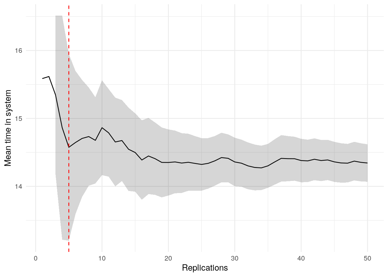
Automated
Description of the algorithm
Using the automated method, an algorithm will tell us the number of runs needed. We will use the ReplicationsAlgorithm class from sim-tools.
Here’s how it works:
- The algorithm runs the simulation model repeatedly, for an increasing number of runs.
- After each run, it checks if the results are stable enough. It does this by looking at the percentage deviation of the confidence interval from the mean.
- The algorithm also incorporates a look-ahead period, meaning it continues to run the simulation and check that results stay stable for the next few runs (and that this wasn’t just a lucky one-off!).
Model adapter
The ReplicationsAlgorithm can be used on a variety of model structures - it just requires a standardised interface, as defined by the ReplicationsAlgorithmModelAdapter class in sim-tools
What this essentially tells us is that the model needs to provide a single_run(replication_number) method, returning results in dictionary form.
@runtime_checkable
class ReplicationsAlgorithmModelAdapter(Protocol):
    """
    Adapter pattern for the "Replications Algorithm".

    All models that use ReplicationsAlgorithm must provide a
    single_run(replication_number) interface.
    """

    def single_run(self, replication_number: int) -> dict[str, float]:
        """
        Run a single unique replication of the model and return results.

        Parameters
        ----------
        replication_number : int
            The replication sequence number.

        Returns
        -------
        dict[str, float]
            {'metric_name': value, ... } for all metrics being tracked.
        """
To achieve this, we wrap our model’s own execution logic inside an adapter class. The SimulationAdapter encapsulates simulation parameters, a runner, and the list of metrics you want to extract. Each call to single_run executes one replication and returns results in the correct dictionary format.
class SimulationAdapter:
    """
    Adapter for running model replications compatible with
    ReplicationsAlgorithm.

    Attributes
    ----------
    param : Parameters
        The simulation parameter object for Runner.
    metrics : list[str]
        The metric(s) to output from each run.
    runner : Runner
        An instance of runner initialised with the provided parameters.
    """
    def __init__(self, param, metrics):
        """
        Initialise adapter.

        Parameters
        ----------
        param : Parameters
            The simulation parameter object for Runner.
        metrics : list[str]
            The metric(s) to output from each run.
        """
        self.param = param
        self.metrics = metrics
        self.runner = Runner(self.param)

    def single_run(self, replication_number):
        """
        Run a single simulation replication and return required metrics.
        """
        result = self.runner.run_single(run=replication_number)
        return {metric: result["run"][metric] for metric in self.metrics}
For example:
adapter = SimulationAdapter(param=Parameters(), metrics=metrics)
adapter.single_run(replication_number=0)
{'mean_wait_time': np.float64(3.227077467801481), 'mean_utilisation_tw': 0.8743911437929205, 'mean_queue_length': 0.6102042855882626, 'mean_time_in_system': np.float64(15.849646506571181), 'mean_patients_in_system': 3.2333777169670244}Run algorithm
We can then use this adapter to run ReplicationsAlgorithm.
# Set up model with adapter
sim_model = SimulationAdapter(
  param=Parameters(warm_up_period=10000,
                   data_collection_period=10000),
  metrics=metrics)

# Set up and run the algorithm
analyser = ReplicationsAlgorithm(
    alpha=0.05,
    half_width_precision=0.1,
    look_ahead=5,
    replication_budget=100,
    verbose=False
)
nreps, summary_frame = analyser.select(model=sim_model, metrics=metrics)
The algorithm returns:
- The number of replications required for each metric (here, assigned to
nreps). - A dataframe containing the cumulative results and deviations for each metric (in a single dataframe, here assigned to
summary_frame).
# View results
print(nreps)
{'mean_wait_time': 24, 'mean_utilisation_tw': 3, 'mean_queue_length': 24, 'mean_time_in_system': 9, 'mean_patients_in_system': 9}HTML(to_html_datatable(summary_frame))| Loading ITables v2.5.2 from the internet... (need help?) |
Again, we can use plotly_confidence_interval_method to create plots.
p = plotly_confidence_interval_method(
    n_reps=nreps["mean_wait_time"],
    conf_ints=summary_frame[
        summary_frame["metric"] == "mean_wait_time"].reset_index(),
    metric_name="Mean Wait Time")
p.update_layout(autosize=True, width=None, height=390)
p = plotly_confidence_interval_method(
n_reps=nreps["mean_utilisation_tw"],
conf_ints=summary_frame[
summary_frame["metric"] == "mean_utilisation_tw"].reset_index(),
metric_name="Mean Utilisation")
p.update_layout(autosize=True, width=None, height=390)p = plotly_confidence_interval_method(
n_reps=nreps["mean_queue_length"],
conf_ints=summary_frame[
summary_frame["metric"] == "mean_queue_length"].reset_index(),
metric_name="Mean Queue Length")
p.update_layout(autosize=True, width=None, height=390)p = plotly_confidence_interval_method(
n_reps=nreps["mean_time_in_system"],
conf_ints=summary_frame[
summary_frame["metric"] == "mean_time_in_system"].reset_index(),
metric_name="Mean Time In System")
p.update_layout(autosize=True, width=None, height=390)p = plotly_confidence_interval_method(
n_reps=nreps["mean_patients_in_system"],
conf_ints=summary_frame[
summary_frame["metric"] == "mean_patients_in_system"].reset_index(),
metric_name="Mean Patients In System")
p.update_layout(autosize=True, width=None, height=390)For this analysis, we have created three R6 classes: WelfordStats, ReplicationTabuliser, and ReplicationsAlgorithm.
NoteView classes
#' Computes running sample mean and variance using Welford's algorithm.
#'
#' @description
#' They are computed via updates to a stored value, rather than storing lots of
#' data and repeatedly taking the mean after new values have been added.
#'
#' Implements Welford's algorithm for updating mean and variance.
#' See Knuth. D `The Art of Computer Programming` Vol 2. 2nd ed. Page 216.
#'
#' This class is based on the Python class `OnlineStatistics` from Tom Monks
#' (2021) sim-tools: fundamental tools to support the simulation process in
#' python (https://github.com/TomMonks/sim-tools) (MIT Licence).
#'
#' @docType class
#' @importFrom R6 R6Class
#'
#' @return Object of `R6Class` with methods for running mean and variance
#' calculation.
#' @export

WelfordStats <- R6Class("WelfordStats", list( # nolint: object_name_linter

  #' @field n Number of observations.
  n = 0L,

  #' @field latest_data Latest data point.
  latest_data = NA,

  #' @field mean Running mean.
  mean = NA,

  #' @field sq Running sum of squares of differences.
  sq = NA,

  #' @field alpha Significance level for confidence interval calculations.
  #' For example, if alpha is 0.05, then the confidence level is 95\%.
  alpha = NA,

  #' @field observer Observer to notify on updates.
  observer = NULL,

  #' @description Initialise the WelfordStats object.
  #' @param data Initial data sample.
  #' @param alpha Significance level for confidence interval calculations.
  #' @param observer Observer to notify on updates.
  #' @return A new `WelfordStats` object.
  initialize = function(data = NULL, alpha = 0.05, observer = NULL) {
    # Set alpha and observer using the provided values/objects
    self$alpha <- alpha
    self$observer <- observer
    # If an initial data sample is supplied, then run update()
    if (!is.null(data)) {
      for (x in as.matrix(data)) {
        self$update(x)
      }
    }
  },

  #' @description Update running statistics with a new data point.
  #' @param x A new data point.
  update = function(x) {
    # Increment counter and save the latest data point
    self$n <- self$n + 1L
    self$latest_data <- x
    # Calculate the mean and sq
    if (self$n == 1L) {
      self$mean <- x
      self$sq <- 0L
    } else {
      updated_mean <- self$mean + ((x - self$mean) / self$n)
      self$sq <- self$sq + ((x - self$mean) * (x - updated_mean))
      self$mean <- updated_mean
    }
    # Update observer if present
    if (!is.null(self$observer)) {
      self$observer$update(self)
    }
  },

  #' @description Computes the variance of the data points.
  variance = function() {
    self$sq / (self$n - 1L)
  },

  #' @description Computes the standard deviation.
  std = function() {
    if (self$n < 3L) return(NA_real_)
    sqrt(self$variance())
  },

  #' @description Computes the standard error of the mean.
  std_error = function() {
    self$std() / sqrt(self$n)
  },

  #' @description Computes the half-width of the confidence interval.
  half_width = function() {
    if (self$n < 3L) return(NA_real_)
    dof <- self$n - 1L
    t_value <- qt(1L - (self$alpha / 2L), df = dof)
    t_value * self$std_error()
  },

  #' @description Computes the lower confidence interval bound.
  lci = function() {
    self$mean - self$half_width()
  },

  #' @description Computes the upper confidence interval bound.
  uci = function() {
    self$mean + self$half_width()
  },

  #' @description Computes the precision of the confidence interval expressed
  #' as the percentage deviation of the half width from the mean.
  deviation = function() {
    mw <- self$mean
    if (is.na(mw) || mw == 0L) return(NA_real_)
    self$half_width() / mw
  }
))
#' Observes and records results from WelfordStats.
#'
#' @description
#' Updates each time new data is processed. Can generate a results dataframe.
#'
#' This class is based on the Python class `ReplicationTabulizer` from Tom
#' Monks (2021) sim-tools: fundamental tools to support the simulation process
#' in python (https://github.com/TomMonks/sim-tools) (MIT Licence).
#'
#' @docType class
#' @importFrom R6 R6Class
#'
#' @return Object of `R6Class` with methods for storing and tabulising results.
#' @export
ReplicationTabuliser <- R6Class("ReplicationTabuliser", list( # nolint: object_name_linter
#' @field data_points List containing each data point.
data_points = NULL,
#' @field cumulative_mean List of the running mean.
cumulative_mean = NULL,
#' @field std List of the standard deviation.
std = NULL,
#' @field lci List of the lower confidence interval bound.
lci = NULL,
#' @field uci List of the upper confidence interval bound.
uci = NULL,
#' @field deviation List of the percentage deviation of the confidence
#' interval half width from the mean.
deviation = NULL,
#' @description Add new results from WelfordStats to the appropriate lists.
#' @param stats An instance of WelfordStats containing updated statistical
#' measures like the mean, standard deviation and confidence intervals.
update = function(stats) {
self$data_points <- c(self$data_points, stats$latest_data)
self$cumulative_mean <- c(self$cumulative_mean, stats$mean)
self$std <- c(self$std, stats$std())
self$lci <- c(self$lci, stats$lci())
self$uci <- c(self$uci, stats$uci())
self$deviation <- c(self$deviation, stats$deviation())
},
#' @description Creates a results table from the stored lists.
#' @return Stored results compiled into a dataframe.
summary_table = function() {
data.frame(
replications = seq_len(length(self$data_points)),
data = self$data_points,
cumulative_mean = self$cumulative_mean,
stdev = self$std,
lower_ci = self$lci,
upper_ci = self$uci,
deviation = self$deviation
)
}
))#' Replication algorithm to automatically select number of replications.
#'
#' @description
#' Implements an adaptive replication algorithm for selecting the
#' appropriate number of simulation replications based on statistical
#' precision.
#'
#' Uses the "Replications Algorithm" from Hoad, Robinson, & Davies (2010).
#' Automated selection of the number of replications for a discrete-event
#' simulation. Journal of the Operational Research Society.
#' https://www.jstor.org/stable/40926090.
#'
#' Given a model's performance measure and a user-set confidence interval
#' half width prevision, automatically select the number of replications.
#' Combines the "confidence intervals" method with a sequential look-ahead
#' procedure to determine if a desired precision in the confidence interval
#' is maintained.
#'
#' This class is based on the Python class `ReplicationsAlgorithm` from Tom
#' Monks (2021) sim-tools: fundamental tools to support the simulation process
#' in python (https://github.com/TomMonks/sim-tools) (MIT Licence).
#'
#' @docType class
#' @importFrom R6 R6Class
#'
#' @return Object of `ReplicationsAlgorithm` with methods for determining the
#' appropriate number of replications to use.
#' @export
ReplicationsAlgorithm <- R6Class("ReplicationsAlgorithm", list( # nolint: object_name_linter
#' @field param Model parameters.
param = NA,
#' @field metrics List of performance measure to track (should correspond to
#' column names from the run results dataframe).
metrics = NA,
#' @field desired_precision The target half width precision for the algorithm
#' (i.e. percentage deviation of the confidence interval from the mean,
#' expressed as a proportion, e.g. 0.1 = 10\%). Choice is fairly arbitrary.
desired_precision = NA,
#' @field initial_replications Number of initial replications to perform.
initial_replications = NA,
#' @field look_ahead Minimum additional replications to look ahead to assess
#' stability of precision. When the number of replications is <= 100, the
#' value of look_ahead is used. When they are > 100, then
#' look_ahead / 100 * max(n, 100) is used.
look_ahead = NA,
#' @field replication_budget Maximum allowed replications. Use for larger
#' models where replication runtime is a constraint.
replication_budget = NA,
#' @field reps Number of replications performed.
reps = NA,
#' @field nreps The minimum number of replicatons required to achieve
#' desired precision for each metric.
nreps = NA,
#' @field summary_table Dataframe containing cumulative statistics for each
#' replication for each metric
summary_table = NA,
#' @description Initialise the ReplicationsAlgorithm object.
#' @param param Model parameters.
#' @param metrics List of performance measure to track.
#' @param desired_precision Target half width precision for the algorithm.
#' @param initial_replications Number of initial replications to perform.
#' @param look_ahead Minimum additional replications to look ahead.
#' @param replication_budget Maximum allowed replications.
#' @param verbose Boolean, whether to print messages about parameters.
initialize = function(
param,
metrics,
desired_precision = 0.1,
initial_replications = 3L,
look_ahead = 5L,
replication_budget = 1000L,
verbose = TRUE
) {
self$param <- param
self$metrics <- metrics
self$desired_precision <- desired_precision
self$initial_replications <- initial_replications
self$look_ahead <- look_ahead
self$replication_budget <- replication_budget
# Initially set reps to the number of initial replications
self$reps <- initial_replications
# Print the parameters
if (isTRUE(verbose)) {
print("Model parameters:") # nolint: print_linter
print(self$param)
}
# Check validity of provided parameters
self$valid_inputs()
},
#' @description
#' Checks validity of provided parameters.
valid_inputs = function() {
for (p in c("initial_replications", "look_ahead")) {
if (self[[p]] %% 1L != 0L || self[[p]] < 0L) {
stop(p, " must be a non-negative integer, but provided ", self[[p]],
".", call. = FALSE)
}
}
if (self$desired_precision <= 0L) {
stop("desired_precision must be greater than 0.", call. = FALSE)
}
if (self$replication_budget < self$initial_replications) {
stop("replication_budget must be less than initial_replications.",
call. = FALSE)
}
},
#' @description
#' Calculate the klimit. Determines the number of additional replications to
#' check after precision is reached, scaling with total replications if they
#' are greater than 100. Rounded down to nearest integer.
#' @return Number of additional replications to verify stability (integer).
klimit = function() {
as.integer((self$look_ahead / 100L) * max(self$reps, 100L))
},
#' @description
#' Find the first position where element is below deviation, and this is
#' maintained through the lookahead period.
#' This is used to correct the ReplicationsAlgorithm, which cannot return
#' a solution below the initial_replications.
#' @param lst List of numbers to compare against desired deviation.
#' @return Integer, minimum replications required to meet and maintain
#' precision.
find_position = function(lst) {
# Ensure that the input is a list
if (!is.list(lst)) {
stop("find_position requires a list but was supplied: ", typeof(lst),
call. = FALSE)
}
# Check if list is empty or no values below threshold
if (length(lst) == 0L || all(is.na(lst)) || !any(unlist(lst) < 0.5)) {
return(NULL)
}
# Find the first non-null value in the list
start_index <- which(!vapply(lst, is.na, logical(1L)))[1L]
# Iterate through the list, stopping when at last point where we still
# have enough elements to look ahead
max_index <- length(lst) - self$look_ahead
if (start_index > max_index) {
return(NULL)
}
for (i in start_index:max_index) {
# Trim to list with current value + lookahead
# Check if all fall below the desired deviation
segment <- lst[i:(i + self$look_ahead)]
if (all(vapply(segment,
function(x) x < self$desired_precision, logical(1L)))) {
return(i)
}
}
return(NULL) # nolint: return_linter
},
#' @description
#' Executes the replication algorithm, determining the necessary number
#' of replications to achieve and maintain the desired precision.
select = function() {
# Create instances of observers for each metric
observers <- setNames(
lapply(self$metrics, function(x) ReplicationTabuliser$new()), self$metrics
)
# Create nested named list to store record for each metric of:
# - nreps (the solution - replications required for precision)
# - target_met (record of how many times in a row the target has been meet,
# used to check if lookahead period has passed)
# - solved (whether it has maintained precision for lookahead)
solutions <- setNames(
lapply(self$metrics, function(x) {
list(nreps = NA, target_met = 0L, solved = FALSE)
}), self$metrics
)
# If there are no initial replications, create empty instances of
# WelfordStats for each metric...
if (self$initial_replications == 0L) {
stats <- setNames(
lapply(
self$metrics, function(x) WelfordStats$new(observer = observers[[x]])
), self$metrics
)
} else {
# If there are, run the replications, then create instances of
# WelfordStats pre-loaded with data from the initial replications... we
# use runner so allows for parallel processing if desired...
self$param[["number_of_runs"]] <- self$initial_replications
result <- runner(self$param)[["run_results"]]
stats <- setNames(
lapply(self$metrics, function(x) {
WelfordStats$new(data = result[[x]], observer = observers[[x]])
}), self$metrics
)
# After completing any replications, check if any have met precision, add
# solution and update count
for (metric in self$metrics) {
if (isTRUE(stats[[metric]]$deviation() < self$desired_precision)) {
solutions[[metric]]$nreps <- self$reps
solutions[[metric]]$target_met <- 1L
# If there is no lookahead, mark as solved
if (self$klimit() == 0L) {
solutions[[metric]]$solved <- TRUE
}
}
}
}
# Whilst have not yet got all metrics marked as solved = TRUE, and still
# under replication budget + lookahead...
is_all_solved <- function(solutions_list) {
statuses <- unlist(lapply(solutions_list, function(x) x$solved))
# If any are NA or FALSE, treat as not solved
all(statuses)
}
while (!is_all_solved(solutions) &&
self$reps < self$replication_budget + self$klimit()) {
# Increment counter
self$reps <- self$reps + 1L
# Run another replication
result <- model(run_number = self$reps,
param = self$param)[["run_results"]]
# Loop through the metrics...
for (metric in self$metrics) {
# If it is not yet solved...
if (!solutions[[metric]]$solved) {
# Update the running statistics for that metric
stats[[metric]]$update(result[[metric]])
# If precision has been achieved...
if (isTRUE(stats[[metric]]$deviation() < self$desired_precision)) {
# Check if target met the time prior - if not, record the solution
if (solutions[[metric]]$target_met == 0L) {
solutions[[metric]]$nreps <- self$reps
}
# Update how many times precision has been met in a row
solutions[[metric]]$target_met <- (
solutions[[metric]]$target_met + 1L
)
# Mark as solved if have finished lookahead period
if (solutions[[metric]]$target_met > self$klimit()) {
solutions[[metric]]$solved <- TRUE
}
} else {
# If precision was not achieved, ensure nreps is None (e.g. in cases
# where precision is lost after a success)
solutions[[metric]]$nreps <- NA
solutions[[metric]]$target_met <- 0L
}
}
}
}
# Correction to result...
for (metric in names(solutions)){
# Use find_position() to check for solution in initial replications
adj_nreps <- self$find_position(as.list(observers[[metric]]$deviation))
# If there was a maintained solution, replace in solutions
if (!is.null(adj_nreps) && !is.na(solutions[[metric]]$nreps)) {
solutions[[metric]]$nreps <- adj_nreps
}
}
# Extract minimum replications for each metric
self$nreps <- lapply(solutions, function(x) x$nreps)
# Extract any metrics that were not solved and return warning
if (anyNA(self$nreps)) {
unsolved <- names(self$nreps)[vapply(self$nreps, is.na, logical(1L))]
warning(
"The replications did not reach the desired precision ",
"for the following metrics - ", toString(unsolved),
call. = FALSE
)
}
# Combine observer summary frames into a single table
summary_tables <- lapply(names(observers), function(name) {
tab <- observers[[name]]$summary_table()
tab$metric <- name
tab
})
self$summary_table <- do.call(rbind, summary_tables)
}
))# Set up algorithm
alg <- ReplicationsAlgorithm$new(
param = create_params(warm_up_period = 10000L,
data_collection_period = 10000L),
metrics = metrics
)[1] "Model parameters:"
$interarrival_time
[1] 5
$consultation_time
[1] 10
$number_of_doctors
[1] 3
$warm_up_period
[1] 10000
$data_collection_period
[1] 10000
$number_of_runs
[1] 5
$verbose
[1] FALSE# Run algorithm
alg$select()
# View recommended number of replications
alg$nreps$mean_wait_time_doctor
[1] 18
$utilisation_doctor
[1] 3
$mean_queue_length_doctor
[1] 19
$mean_time_in_system
[1] 5
$mean_patients_in_system
[1] 6# View full results table
alg$summary_table |>
kable() |>
scroll_box(height = "400px")| replications | data | cumulative_mean | stdev | lower_ci | upper_ci | deviation | metric |
|---|---|---|---|---|---|---|---|
| 1 | 5.6676719 | 5.6676719 | NA | NA | NA | NA | mean_wait_time_doctor |
| 2 | 5.3283685 | 5.4980202 | NA | NA | NA | NA | mean_wait_time_doctor |
| 3 | 4.9340038 | 5.3100147 | 0.3671783 | 4.3978934 | 6.2221361 | 0.1717738 | mean_wait_time_doctor |
| 4 | 3.6718311 | 4.9004688 | 0.8722335 | 3.5125507 | 6.2883870 | 0.2832215 | mean_wait_time_doctor |
| 5 | 3.4128133 | 4.6029377 | 1.0065869 | 3.3530950 | 5.8527805 | 0.2715315 | mean_wait_time_doctor |
| 6 | 5.0599633 | 4.6791087 | 0.9194487 | 3.7142064 | 5.6440109 | 0.2062150 | mean_wait_time_doctor |
| 7 | 4.8427498 | 4.7024860 | 0.8416138 | 3.9241231 | 5.4808489 | 0.1655216 | mean_wait_time_doctor |
| 8 | 4.8621394 | 4.7224426 | 0.7812248 | 4.0693224 | 5.3755629 | 0.1383014 | mean_wait_time_doctor |
| 9 | 4.6672848 | 4.7163140 | 0.7310001 | 4.1544175 | 5.2782104 | 0.1191389 | mean_wait_time_doctor |
| 10 | 6.0724262 | 4.8519252 | 0.8117215 | 4.2712546 | 5.4325958 | 0.1196784 | mean_wait_time_doctor |
| 11 | 4.2691492 | 4.7989456 | 0.7898594 | 4.2683108 | 5.3295803 | 0.1105732 | mean_wait_time_doctor |
| 12 | 3.4126731 | 4.6834229 | 0.8528233 | 4.1415648 | 5.2252810 | 0.1156970 | mean_wait_time_doctor |
| 13 | 4.8910189 | 4.6993918 | 0.8185437 | 4.2047508 | 5.1940328 | 0.1052564 | mean_wait_time_doctor |
| 14 | 3.4921984 | 4.6131637 | 0.8500401 | 4.1223651 | 5.1039622 | 0.1063909 | mean_wait_time_doctor |
| 15 | 3.8903965 | 4.5649792 | 0.8401085 | 4.0997426 | 5.0302158 | 0.1019143 | mean_wait_time_doctor |
| 16 | 2.9905528 | 4.4665776 | 0.9020290 | 3.9859202 | 4.9472349 | 0.1076120 | mean_wait_time_doctor |
| 17 | 5.3595945 | 4.5191080 | 0.8998408 | 4.0564525 | 4.9817634 | 0.1023776 | mean_wait_time_doctor |
| 18 | 3.8887614 | 4.4840887 | 0.8855267 | 4.0437267 | 4.9244508 | 0.0982055 | mean_wait_time_doctor |
| 19 | 3.6892115 | 4.4422531 | 0.8796859 | 4.0182580 | 4.8662481 | 0.0954459 | mean_wait_time_doctor |
| 20 | 4.2884182 | 4.4345613 | 0.8569141 | 4.0335132 | 4.8356095 | 0.0904369 | mean_wait_time_doctor |
| 21 | 4.3597185 | 4.4309974 | 0.8353762 | 4.0507387 | 4.8112561 | 0.0858179 | mean_wait_time_doctor |
| 22 | 3.8827551 | 4.4060773 | 0.8235803 | 4.0409222 | 4.7712323 | 0.0828753 | mean_wait_time_doctor |
| 23 | 4.6397718 | 4.4162379 | 0.8061191 | 4.0676459 | 4.7648299 | 0.0789342 | mean_wait_time_doctor |
| 1 | 0.6832362 | 0.6832362 | NA | NA | NA | NA | utilisation_doctor |
| 2 | 0.7014341 | 0.6923351 | NA | NA | NA | NA | utilisation_doctor |
| 3 | 0.6503975 | 0.6783559 | 0.0258659 | 0.6141014 | 0.7426104 | 0.0947210 | utilisation_doctor |
| 4 | 0.6437990 | 0.6697167 | 0.0272869 | 0.6262971 | 0.7131363 | 0.0648327 | utilisation_doctor |
| 5 | 0.6789189 | 0.6715571 | 0.0239868 | 0.6417735 | 0.7013407 | 0.0443500 | utilisation_doctor |
| 6 | 0.6713653 | 0.6715251 | 0.0214546 | 0.6490099 | 0.6940404 | 0.0335285 | utilisation_doctor |
| 7 | 0.6775094 | 0.6723800 | 0.0197155 | 0.6541463 | 0.6906138 | 0.0271182 | utilisation_doctor |
| 8 | 0.6528520 | 0.6699390 | 0.0195151 | 0.6536240 | 0.6862541 | 0.0243530 | utilisation_doctor |
| 1 | 1.2047321 | 1.2047321 | NA | NA | NA | NA | mean_queue_length_doctor |
| 2 | 1.0585763 | 1.1316542 | NA | NA | NA | NA | mean_queue_length_doctor |
| 3 | 1.0061322 | 1.0898135 | 0.1029189 | 0.8341487 | 1.3454783 | 0.2345950 | mean_queue_length_doctor |
| 4 | 0.7220796 | 0.9978800 | 0.2021598 | 0.6761987 | 1.3195614 | 0.3223648 | mean_queue_length_doctor |
| 5 | 0.7147191 | 0.9412479 | 0.2160728 | 0.6729580 | 1.2095377 | 0.2850363 | mean_queue_length_doctor |
| 6 | 0.9998528 | 0.9510153 | 0.1947367 | 0.7466517 | 1.1553790 | 0.2148900 | mean_queue_length_doctor |
| 7 | 0.9630582 | 0.9527358 | 0.1778278 | 0.7882725 | 1.1171990 | 0.1726221 | mean_queue_length_doctor |
| 8 | 0.9401393 | 0.9511612 | 0.1646967 | 0.8134713 | 1.0888511 | 0.1447598 | mean_queue_length_doctor |
| 9 | 0.9319599 | 0.9490277 | 0.1541926 | 0.8305048 | 1.0675506 | 0.1248888 | mean_queue_length_doctor |
| 10 | 1.2095963 | 0.9750846 | 0.1671025 | 0.8555466 | 1.0946225 | 0.1225924 | mean_queue_length_doctor |
| 11 | 0.8724811 | 0.9657570 | 0.1615177 | 0.8572479 | 1.0742660 | 0.1123565 | mean_queue_length_doctor |
| 12 | 0.6465119 | 0.9391532 | 0.1794699 | 0.8251235 | 1.0531830 | 0.1214176 | mean_queue_length_doctor |
| 13 | 0.9578633 | 0.9405925 | 0.1719077 | 0.8367097 | 1.0444752 | 0.1104440 | mean_queue_length_doctor |
| 14 | 0.7166333 | 0.9245954 | 0.1756750 | 0.8231637 | 1.0260271 | 0.1097039 | mean_queue_length_doctor |
| 15 | 0.7937702 | 0.9158737 | 0.1726219 | 0.8202789 | 1.0114685 | 0.1043755 | mean_queue_length_doctor |
| 16 | 0.5950870 | 0.8958245 | 0.1850493 | 0.7972187 | 0.9944304 | 0.1100727 | mean_queue_length_doctor |
| 17 | 1.0952642 | 0.9075563 | 0.1855878 | 0.8121358 | 1.0029767 | 0.1051400 | mean_queue_length_doctor |
| 18 | 0.7925600 | 0.9011676 | 0.1820754 | 0.8106236 | 0.9917116 | 0.1004741 | mean_queue_length_doctor |
| 19 | 0.7424607 | 0.8928146 | 0.1806527 | 0.8057428 | 0.9798864 | 0.0975251 | mean_queue_length_doctor |
| 20 | 0.8539327 | 0.8908705 | 0.1760492 | 0.8084769 | 0.9732641 | 0.0924866 | mean_queue_length_doctor |
| 21 | 0.8341843 | 0.8881712 | 0.1720368 | 0.8098609 | 0.9664814 | 0.0881702 | mean_queue_length_doctor |
| 22 | 0.7866429 | 0.8835562 | 0.1692804 | 0.8085015 | 0.9586110 | 0.0849462 | mean_queue_length_doctor |
| 23 | 0.9277437 | 0.8854774 | 0.1656448 | 0.8138472 | 0.9571076 | 0.0808944 | mean_queue_length_doctor |
| 24 | 0.7972331 | 0.8818006 | 0.1630022 | 0.8129708 | 0.9506304 | 0.0780559 | mean_queue_length_doctor |
| 1 | 15.5867030 | 15.5867030 | NA | NA | NA | NA | mean_time_in_system |
| 2 | 15.6470504 | 15.6168767 | NA | NA | NA | NA | mean_time_in_system |
| 3 | 14.8030177 | 15.3455904 | 0.4708495 | 14.1759353 | 16.5152455 | 0.0762209 | mean_time_in_system |
| 4 | 13.4202268 | 14.8642495 | 1.0366078 | 13.2147752 | 16.5137238 | 0.1109692 | mean_time_in_system |
| 5 | 13.4190380 | 14.5752072 | 1.1061844 | 13.2016978 | 15.9487166 | 0.0942360 | mean_time_in_system |
| 6 | 14.9968766 | 14.6454854 | 1.0042656 | 13.5915733 | 15.6993975 | 0.0719616 | mean_time_in_system |
| 7 | 15.0665982 | 14.7056444 | 0.9304792 | 13.8450947 | 15.5661941 | 0.0585183 | mean_time_in_system |
| 8 | 14.9253467 | 14.7331072 | 0.8649513 | 14.0099898 | 15.4562245 | 0.0490811 | mean_time_in_system |
| 9 | 14.2334536 | 14.6775901 | 0.8260523 | 14.0426301 | 15.3125501 | 0.0432605 | mean_time_in_system |
| 10 | 16.5390912 | 14.8637402 | 0.9762495 | 14.1653734 | 15.5621070 | 0.0469846 | mean_time_in_system |
| 1 | 3.2207992 | 3.2207992 | NA | NA | NA | NA | mean_patients_in_system |
| 2 | 3.2002959 | 3.2105475 | NA | NA | NA | NA | mean_patients_in_system |
| 3 | 2.9105293 | 3.1105415 | 0.1735187 | 2.6794971 | 3.5415858 | 0.1385753 | mean_patients_in_system |
| 4 | 2.6581309 | 2.9974388 | 0.2669107 | 2.5727244 | 3.4221533 | 0.1416925 | mean_patients_in_system |
| 5 | 2.7277981 | 2.9435107 | 0.2607148 | 2.6197905 | 3.2672309 | 0.1099776 | mean_patients_in_system |
| 6 | 3.0399497 | 2.9595838 | 0.2364907 | 2.7114021 | 3.2077656 | 0.0838570 | mean_patients_in_system |
| 7 | 2.9924023 | 2.9642722 | 0.2162415 | 2.7642821 | 3.1642623 | 0.0674668 | mean_patients_in_system |
| 8 | 2.9064020 | 2.9570384 | 0.2012436 | 2.7887946 | 3.1252822 | 0.0568961 | mean_patients_in_system |
| 9 | 2.9145095 | 2.9523130 | 0.1887791 | 2.8072045 | 3.0974215 | 0.0491508 | mean_patients_in_system |
| 10 | 3.2673469 | 2.9838164 | 0.2039668 | 2.8379073 | 3.1297255 | 0.0489002 | mean_patients_in_system |
| 11 | 2.7941860 | 2.9665773 | 0.2017704 | 2.8310261 | 3.1021284 | 0.0456928 | mean_patients_in_system |
We can use the function plot_replication_ci from above again to create the plots.
plot_replication_ci(
  conf_ints = filter(alg$summary_table, metric == "mean_wait_time_doctor"),
  yaxis_title = "Mean wait time",
  min_rep = alg$nreps[["mean_wait_time_doctor"]]
)
Warning: Removed 2 rows containing missing values or values outside the scale range
(`geom_ribbon()`).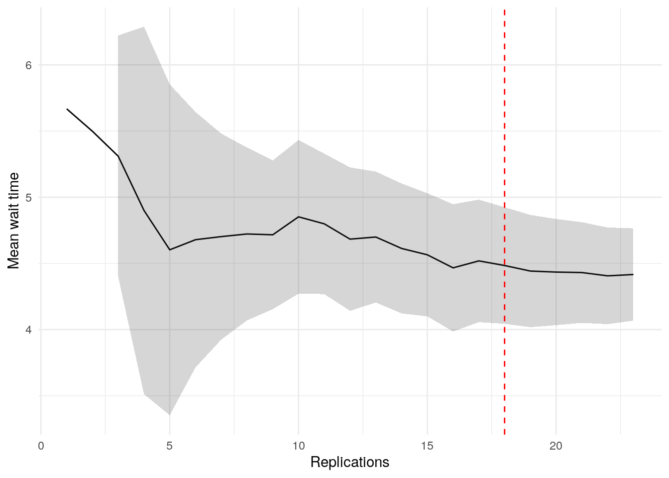
plot_replication_ci(
  conf_ints = filter(alg$summary_table, metric == "utilisation_doctor"),
  yaxis_title = "Mean utilisation",
  min_rep = alg$nreps[["utilisation_doctor"]]
)
Warning: Removed 2 rows containing missing values or values outside the scale range
(`geom_ribbon()`).
plot_replication_ci(
  conf_ints = filter(alg$summary_table, metric == "mean_queue_length_doctor"),
  yaxis_title = "Mean queue length",
  min_rep = alg$nreps[["mean_queue_length_doctor"]]
)
Warning: Removed 2 rows containing missing values or values outside the scale range
(`geom_ribbon()`).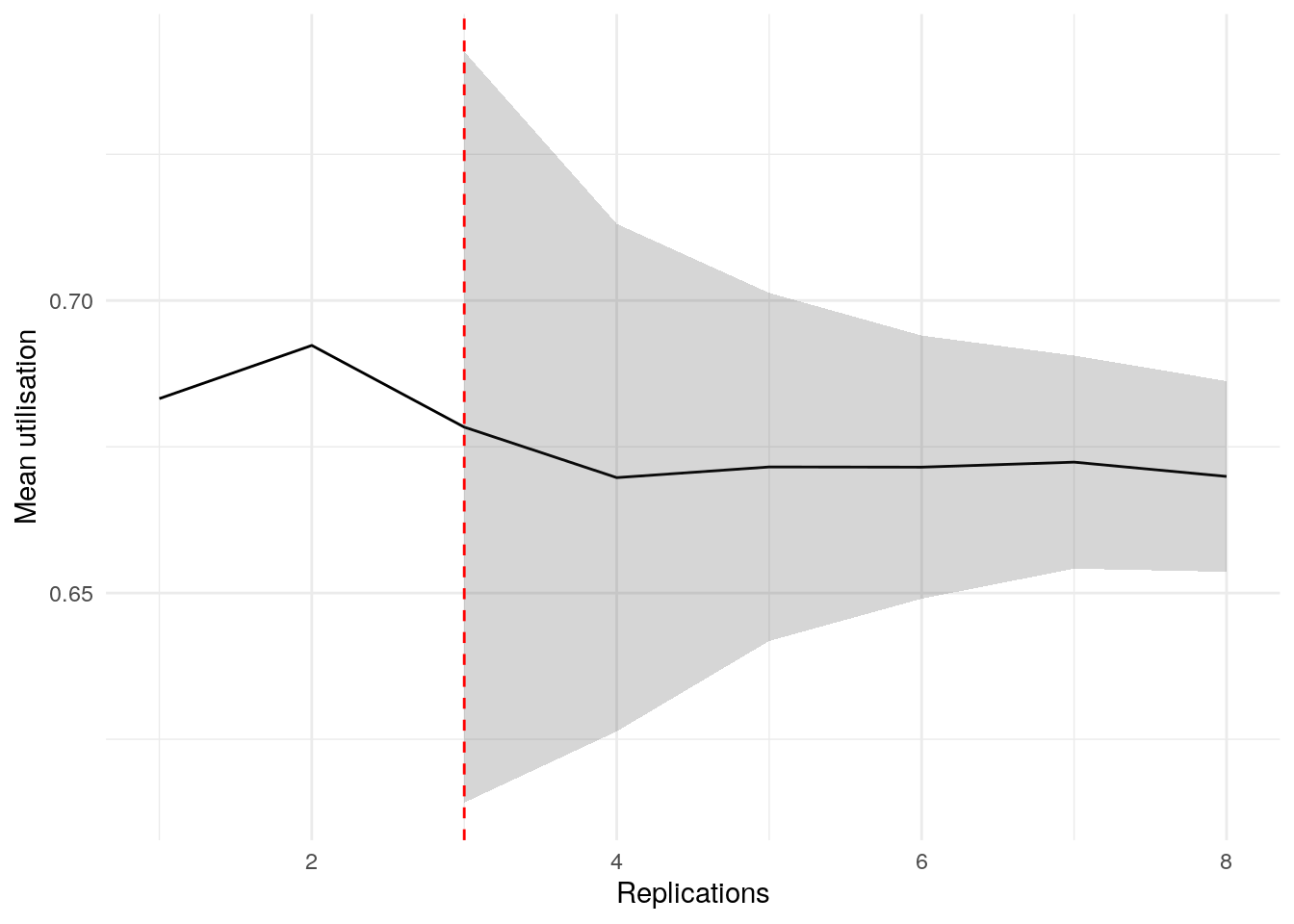
plot_replication_ci(
  conf_ints = filter(alg$summary_table, metric == "mean_time_in_system"),
  yaxis_title = "Mean time in system",
  min_rep = alg$nreps[["mean_time_in_system"]]
)
Warning: Removed 2 rows containing missing values or values outside the scale range
(`geom_ribbon()`).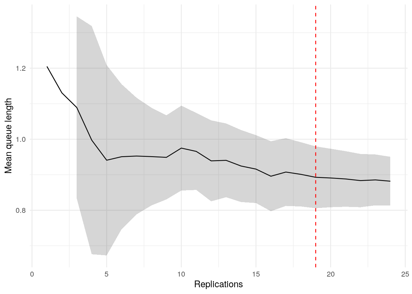
plot_replication_ci(
  conf_ints = filter(alg$summary_table, metric == "mean_patients_in_system"),
  yaxis_title = "Mean patients in system",
  min_rep = alg$nreps[["mean_patients_in_system"]]
)
Warning: Removed 2 rows containing missing values or values outside the scale range
(`geom_ribbon()`).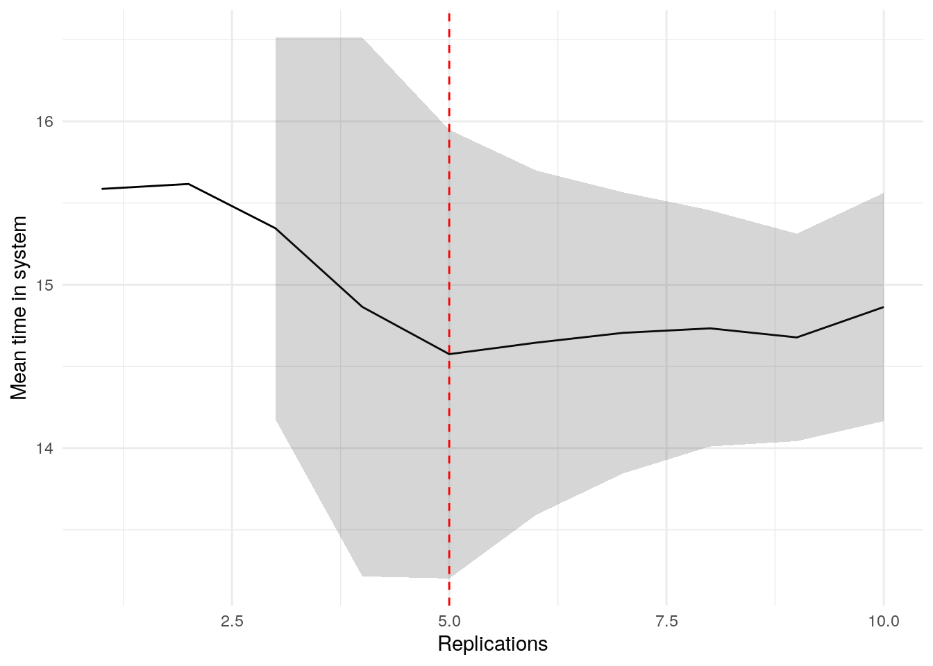
Explore the example models
Nurse visit simulation
![]() Click to visit pydesrap_mms repository
Click to visit pydesrap_mms repository
| Key files | simulation/SimulationAdapternotebooks/choosing_replications.ipynb |
| What to look for? | Runs the manual and automated methods, as on this page. Includes a sensitivity analysis which checks the stability of the suggested number of replications, achieved by adding a seed_offset parameter that can be used to create a new set of seeds. The variation observed in the sensitivity analysis influences the chosen number of replications, and this is worth being aware of, if you also find yourself with a simulation with a relatively low suggested number of replications. |
![]() Click to visit rdesrap_mms repository
Click to visit rdesrap_mms repository
| Key files | R/choose_replications.Rrmarkdown/choosing_replications.md |
| What to look for? | Runs the manual and automated methods, as on this page. Includes a sensitivity analysis which checks the stability of the suggested number of replications, achieved by adding a seed_offset parameter that can be used to create a new set of seeds. The variation observed in the sensitivity analysis influences the chosen number of replications, and this is worth being aware of, if you also find yourself with a simulation with a relatively low suggested number of replications. |
Stroke pathway simulation
Not relevant - replicating an existing model described in a paper, so just used the number of replications stated by the authors.
Test yourself
Have a go for yourself!
Try out both the manual and automated methods described above to work out how many replications you need for your own simulation model.
See what happens if you change model parameters like run length - notice how this affects the recommended number of replications.