import os
from IPython.display import HTML
from itables import to_html_datatable
import numpy as np
import pandas as pd
import plotly.express as px
import plotly.graph_objects as go
import scipy.stats as st
import simpy
from sim_tools.distributions import ExponentialLength of warm-up
Learning objectives:
- Learn about the time series inspection approach.
- Understand how to implement this approach.
Pre-reading:
This page continues on from: Replications.
Entity generation → Entity processing → Initialisation bias → Performance measures → Replications → Length of warm-up
Required packages:
These should be available from environment setup in the “Test yourself” section of Environments.
library(dplyr)
library(ggplot2)
library(gridExtra)
library(knitr)
library(plotly)
library(R6)
library(simmer)
library(tidyr)Determining a suitable length of warm-up
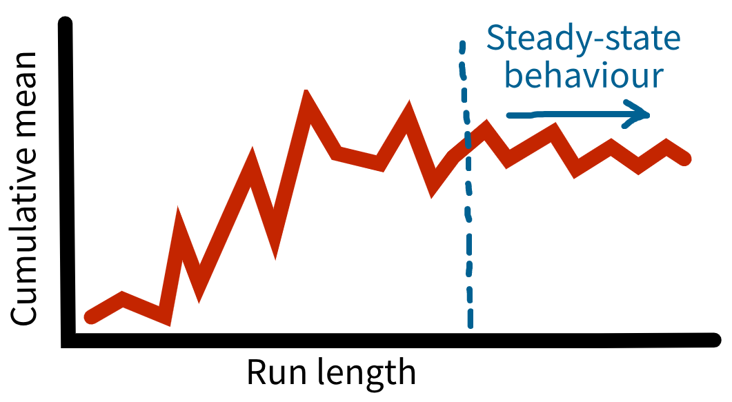
A warm-up period helps address initialisation bias, which occurs when a simulation begins in an “empty” state that doesn’t reflect how the real system usually operates. In this early phase, performance measures can be unusually high or low because the system hasn’t yet settled into typical conditions. Running the model for a warm-up period before collecting results allows it to reach steady-state behaviour - a stage where performance measures are stable and represent typical, ongoing behaviour.
Many different methods have been proposed for determining a suitable length of warm-up - the simplest is the time series inspection approach. This involves looking at performance measures over time to identify when the system is exhibiting steady state behaviour (even though the system will never truly reach a “steady state”).
We could plot mean results over time, but this would fluctuate too much. Instead, we plot the cumulative mean of the performance measures over time. We then look for the point where this smoothes out and stabilises - this indicates where your warm-up period should end (Robinson (2007)).
When determining your warm-up period, you should:
- Run the model with multiple replications (at least five) (Robinson (2007)).
- Use a long run length (e.g., 5-10 times your planned simulation length).
- Use your base case parameters (and, if these changes, re-assess the appropriate warm-up period).
Choice of an appropriate warm-up length forms part of your model experimentation validation (see verification and validation page).
Implementing the time series inspection approach
It’s important to include all relevant metrics when implementing this approach. For our model, that means:
- Mean wait time
- Mean doctor utilisation
- Mean queue length
- Mean time in system
- Mean number of patients in system
Why not other metrics?
- Total arrivals: Not impacted by initialisation bias
- Mean time in consultation: Not impacted by initialisation bias
- Unseen (backlogged) patients: In the current model set-up, number of unseen patients is very low or zero, so this is not that useful in our consideration of initialisation bias. However, if your model configuration leads to significant backlogs, this metric could become relevant for warm-up analysis.
For this approach, we need to track the performance measures as the simulation runs. This allows us to identify when the system reaches steady state. There are a few ways you might consider implementing this.
Approach 1. Extract data from existing lists
During the simulation run, many performance measures are already recorded and stored in lists, along with their corresponding event times. We could extract and process these but:
- ❌ Requires extensive changes to
Runner- in particular, to extract time-weighted metrics during the run. These require helper methods to compute and summarise the metrics. Other methods are needed to process and output the results. - ❌
Runnerbecomes quite cluttered - it then contains code to execute replications, aggregate final results, and now to handle time-series extraction and processing (when we only need this code for this analysis, and not anything else). - ❌ This would collect data from every event (potentially tens-of-thousands of timepoints!). For warm-up analysis, collecting data at regular intervals is sufficient.
Approach 2. Separate WarmupAuditor class
We can create a dedicated WarmupAuditor class that runs in parallel with the simulation. It samples performance measures at regular intervals. Benefits of this approach are:
- ✅ No changes needed to the original simulation code (
Model,Runner,Parameters, etc.). - ✅ All warm-up analysis logic is separate and self-contained, making it easier to understand, maintain, reuse or remove as needed.
- ✅ Data is collected efficiently - only at the required intervals, not every event - producing smaller, more manageable datasets.
This is the approach we have used.
Acknowledgements: This auditor-based strategy is adapted from Tom Monks (2024) Lab 6 Output Analysis in HPDM097 - Making a difference with health data (MIT Licence).
Approach 3. Adding audit methods to Model
You might be tempted to implement the warm-up auditor as a method within Model, but we would recommend against this.
- ❌
Modelbecomes quite cluttered - it should represent core simulation logic (patient arrivals, resource usage, etc.) - but now also have warm-up analysis methods mixed in. - ❌ This analysis is only performed during initial model development, and not during production runs or scenario analysis, so there is no need for it to be in the main model definition.
Simulation code
The simulation being used is that from the Replications page.
Auditor class
The WarmupAuditor class is created by passing a Model instance and an interval (in minutes). The run() method starts both the auditor process (using self.model.env.process()) and the simulation (self.model.run()).
The audit process _audit_model() runs continuously throughout the simulation, collecting performance measures at the specified intervals. It calls dedicated methods for each metric that calculate the cumulative mean at that timepoint (e.g., _get_wait_time(), _get_utilisation()).
The results are stored as a list of dictionaries in audit_results, with one entry per interval containing the simulation time and all five performance measures.
class WarmupAuditor():
"""
Warm-up auditor for the model.
Records cumulative mean results at regular intervals.
Attributes
----------
model : Model
Instance of Model() to run the simulation.
interval : int
Audit frequency (minutes).
audit_results : list
List of dictionaries containing audit snapshots at each interval.
current_time : int
Current simulation time to perform audit.
"""
def __init__(self, model, interval):
"""
Initialise auditor.
Parameters
----------
model : Model
Instance of Model() to run the simulation.
interval : int
Audit frequency (minutes).
"""
self.model = model
self.interval = interval
self.audit_results = []
self.current_time = np.nan
def run(self):
"""
Run auditor alongside simulation model.
"""
self.model.env.process(self._audit_model())
self.model.run()
def _audit_model(self):
"""
Audit the model at the specified intervals.
"""
while True:
self.current_time = self.model.env.now
self.audit_results.append({
"time": self.current_time,
"wait_time": self._get_wait_time(),
"time_in_system": self._get_time_in_system(),
"queue_length": self._get_queue_length(),
"utilisation": self._get_utilisation(),
"patients_in_system": self._get_patients_in_system()
})
yield self.model.env.timeout(self.interval)
def _get_wait_time(self):
"""
Compute mean wait time for patients seen by current time.
Returns
-------
float
Mean wait time across all patients who have been seen.
"""
wait_times = [
patient.wait_time
for patient in self.model.patients
if not np.isnan(patient.wait_time)
]
if wait_times:
return np.mean(wait_times)
return np.nan
def _get_time_in_system(self):
"""
Compute mean time in system (for patients completed by current time).
Returns
-------
float
Mean time in system for patients completed by current time.
"""
time_in_system = []
for patient in self.model.patients:
if not np.isnan(patient.end_time):
time_in_system.append(patient.end_time - patient.arrival_time)
if time_in_system:
return np.mean(time_in_system)
return np.nan
def _get_queue_length(self):
"""
Compute time-weighted mean queue length up to current time.
Returns
-------
float
Time-weighted mean queue length from start to current time.
"""
total_area = sum(self.model.doctor.area_n_in_queue)
if self.current_time > 0:
return total_area / self.current_time
return 0
def _get_utilisation(self):
"""
Compute time-weighted mean utilisation up to current time.
Returns
-------
float
Time-weighted mean utilisation from start to current time.
"""
total_area = sum(self.model.doctor.area_resource_busy)
total_capacity = self.model.param.number_of_doctors * self.current_time
if self.current_time > 0:
return total_area / total_capacity
return 0
def _get_patients_in_system(self):
"""
Computer time-weighted mean patients in system up to current time.
Returns
-------
float
Time-weighted mean patients in system from start to current time.
"""
total_area = sum(self.model.area_n_in_system)
if self.current_time > 0:
return total_area / self.current_time
return 0Run model with auditor
It’s important to run the time series inspection on results from multiple replications. The run_warmup_analysis() function executes WarmupAuditor for the specified number of replications, and returns the results as a single dataframe.
def run_warmup_analysis(
audit_interval, data_collection_period, number_of_runs
):
"""
Runs the model without a warm-up, collecting performance measures at
regular intervals, used to determine appropriate length of warm-up.
Parameters
----------
audit_interval : int
Audit frequency (minutes).
data_collection_period : int
Duration of the data collection period (minutes).
number_of_runs : int
The number of runs (i.e., replications).
Returns
-------
pd.DataFrame
Combined results from all replications.
"""
# Fixed set of parameters for all runs
# Important: Sets warm-up period to zero
param = Parameters(
warm_up_period=0,
data_collection_period=data_collection_period
)
# Store results from each replication
all_dfs = []
# Loop through replications
for run in range(number_of_runs):
# Run model with auditor
model = Model(param=param, run_number=run)
auditor = WarmupAuditor(model=model, interval=audit_interval)
auditor.run()
# Convert the run's audit results to DataFrame
run_df = pd.DataFrame(auditor.audit_results)
run_df["run"] = run
all_dfs.append(run_df)
# Combine all runs into a single DataFrame
return pd.concat(all_dfs, ignore_index=True)audit_results = run_warmup_analysis(
audit_interval=10,
data_collection_period=14400,
number_of_runs=10
)
# Preview audit results
HTML(to_html_datatable(audit_results.head(200)))| Loading ITables v2.5.2 from the internet... (need help?) |
Plot the results for time series inspection
We can now create plots of the cumulative mean metrics over time. We plot the results from each run (light blue), then an overall cumulative mean (dark blue). Rather than attempting to properly combine time-weighted statistics across runs with different event timepoints, we:
- Pool all timepoint observations from all runs
- Sort them chronologically
- Compute a running average of the cumulative mean values
Whilst this is just an approximation of the cumulative mean for time-weighted values, it is perfectly fine for the purposes of this exercise, which is just so see roughly when metrics stabilise.
def plot_time_series(audit_results, metric, warmup_time=None):
"""
Plot cumulative mean trajectories and compute overall cumulative mean.
Parameters
----------
audit_results : pd.DataFrame
Audit results, where columns include "time", "run" and the
chosen metric like "wait_time" or "time_in_system".
metric : str
The performance measure to visualise.
warmup_time : int
The time point at which to display a vertical dashed line marking the
suggested warm-up period.
Returns
-------
plotly.graph_objects.Figure
A Plotly Figure object containing cumulative mean trajectories for
each run and the overall cumulative mean.
"""
# Computer overall cumulative mean
df = audit_results.groupby("time")[metric].mean().reset_index()
df["overall_cumulative"] = df[metric].expanding().mean()
# Plot cumulative mean for each run
fig = px.line(
data_frame=audit_results,
x="time",
y=metric,
line_group="run"
)
fig.update_traces(line_color="lightblue")
# Overlay overall cumulative mean
overall_fig = px.line(df, x="time", y="overall_cumulative")
fig.add_traces(list(overall_fig.select_traces()))
# Add warm-up line
if warmup_time:
fig.add_vline(x=warmup_time, line_color="red", line_dash="dash",
annotation_text="Suggested warm-up",
annotation_font_color="red",
annotation_position="top right")
# Axis labels and layout
fig.update_layout(
xaxis_title="Run time (minutes)",
yaxis_title=f"cumulative_mean_{metric}",
template="plotly_white"
)
return figplot_time_series(audit_results, "wait_time", 3000)plot_time_series(audit_results, "utilisation", 3000)plot_time_series(audit_results, "queue_length", 3000)plot_time_series(audit_results, "time_in_system", 3000)plot_time_series(audit_results, "patients_in_system", 3000)Simulation code
The simulation being used and edited on this page is that from the Replications page.
The parameter, warm-up, run results, model and runner functions are unchanged. However, we do need to make a change to the function used to calculate utilisation
Functions to calculate different metrics
We will re-use the calc_utilisation function to calculate utilisation at each timepoint. To enable this, we need to add a new argument: groups.
Previously we just grouped by resource, but we now want to also group by replication (as we are processing a full results table containing multiple replications).
#' Calculate the resource utilisation
#'
#' Utilisation is given by the total effective usage time (`in_use`) over
#' the total time intervals considered (`dt`).
#'
#' Credit: The utilisation calculation is adapted from the
#' `plot.resources.utilization()` function in simmer.plot 0.1.18, which is
#' shared under an MIT Licence (Ucar I, Smeets B (2023). simmer.plot: Plotting
#' Methods for 'simmer'. https://r-simmer.org
#' https://github.com/r-simmer/simmer.plot.).
#'
#' @param resources Dataframe with times patients use or queue for resources.
#' @param simulation_end_time Time at end of simulation run.
#' @param groups Optional list of columns to group by for the calculation.
#' @param summarise If TRUE, return overall utilisation. If FALSE, just return
#' the resource dataframe with the additional columns interval_duration,
#' effective_capacity and utilisation.
#'
#' @importFrom dplyr across group_by mutate n row_number summarise ungroup
#' @importFrom rlang .data
#' @importFrom tidyr pivot_wider
#' @importFrom tidyselect all_of
#'
#' @return Tibble with columns containing result for each resource.
#' @export
calc_utilisation <- function(
resources, simulation_end_time, groups = NULL, summarise = TRUE
) {
# Create list of grouping variables (always "resource" but can add others)
group_vars <- c("resource", groups)
# Calculate utilisation
util_df <- resources |>
group_by(across(all_of(group_vars))) |>
mutate(
# Calculate time between this row and the next. For final row,
# lead(time) returns NA, so use simulation_end_time - time
interval_duration = ifelse(
row_number() == n(),
simulation_end_time - .data[["time"]],
lead(.data[["time"]]) - .data[["time"]]
),
# Ensures effective capacity is never less than number of servers in
# use (in case of situations where servers may exceed "capacity").
effective_capacity = pmax(.data[["capacity"]], .data[["server"]]),
# Divide number of servers in use by effective capacity
# Set to NA if effective capacity is 0
utilisation = ifelse(.data[["effective_capacity"]] > 0L,
.data[["server"]] / .data[["effective_capacity"]],
NA_real_)
)
# If summarise = TRUE, find total utilisation
if (summarise) {
util_df |>
summarise(
# Multiply each utilisation by its own unique duration. The total of
# those is then divided by the total duration of all intervals.
# Hence, we are calculated a time-weighted average utilisation.
utilisation = (sum(.data[["utilisation"]] *
.data[["interval_duration"]], na.rm = TRUE) /
sum(.data[["interval_duration"]], na.rm = TRUE))
) |>
pivot_wider(names_from = "resource",
values_from = "utilisation",
names_glue = "utilisation_{resource}") |>
ungroup()
} else {
# If summarise = FALSE, just return the util_df with no further processing
ungroup(util_df)
}
}Time series inspection function
We have a new time_series_inspection function for this analysis, which is explained line-by-line below.
#' Time series inspection method for determining length of warm-up.
#'
#' Find the cumulative mean results and plot over time (overall and per run).
#'
#' @param result Named list with `arrivals` containing output from
#' `get_mon_arrivals()` and `resources` containing output from
#' `get_mon_resources()` (`per_resource = TRUE` and `ongoing = TRUE`).
#' @param simulation_end_time Time at end of simulation run.
#' @param file_path Path to save figure to.
#' @param warm_up Location on X axis to plot vertical red line indicating the
#' chosen warm-up period. Defaults to NULL, which will not plot a line.
#'
#' @importFrom dplyr rename
#' @importFrom ggplot2 ggplot geom_line aes_string labs theme_minimal
#' @importFrom ggplot2 geom_vline annotate ggsave
#' @importFrom gridExtra marrangeGrob
#' @importFrom rlang .data
#'
#' @export
time_series_inspection <- function(
result, simulation_end_time, file_path, warm_up = NULL
) {
# Set up lists
plot_list <- list()
metrics <- list()
# Wait time of each patient at each timepoint
metrics[[1L]] <- result[["arrivals"]] |>
rename(time = .data[["serve_start"]]) |>
dplyr::select(all_of(c("replication", "time", "wait_time")))
# Utilisation at each timepoint
metrics[[2L]] <- calc_utilisation(result[["resources"]],
simulation_end_time = simulation_end_time,
groups = c("resource", "replication"),
summarise = FALSE) |>
dplyr::select(all_of(c("replication", "time", "utilisation")))
# Queue length at each timepoint
metrics[[3L]] <- result[["arrivals"]] |>
rename(time = .data[["start_time"]]) |>
dplyr::select(all_of(c("replication", "time", "queue_on_arrival")))
# Time in system at each timepoint
metrics[[4L]] <- result[["arrivals"]] |>
rename(time = .data[["start_time"]]) |>
dplyr::select(all_of(c("replication", "time", "time_in_system")))
# Patients in system at each timepoint
metrics[[5L]] <- rename(result[["patients_in_system"]],
patients_in_system = .data[["count"]])
# Loop through all the dataframes in df_list
for (i in seq_along(metrics)) {
# Get name of the metric
metric <- setdiff(names(metrics[[i]]), c("time", "replication"))
# Calculate cumulative mean for the current metric
cumulative <- metrics[[i]] |>
arrange(.data[["replication"]], .data[["time"]]) |>
group_by(.data[["replication"]]) |>
mutate(cumulative_mean = cumsum(.data[[metric]]) /
seq_along(.data[[metric]])) |>
ungroup()
# Repeat calculation, but including all replications in one
overall_cumulative <- metrics[[i]] |>
arrange(.data[["time"]]) |>
mutate(cumulative_mean = cumsum(.data[[metric]]) /
seq_along(.data[[metric]])) |>
ungroup()
# Create plot
p <- ggplot() +
geom_line(data = cumulative,
aes(x = time, y = cumulative_mean, group = replication), # nolint
color = "lightblue", alpha = 0.8) +
geom_line(data = overall_cumulative,
aes(x = time, y = cumulative_mean),
color = "darkblue") +
labs(x = "Run time (minutes)", y = paste("Cumulative mean", metric)) +
theme_minimal()
# Add line to indicate suggested warm-up length if provided
if (!is.null(warm_up)) {
p <- p +
geom_vline(xintercept = warm_up, linetype = "dashed", color = "red") +
annotate("text", x = warm_up, y = Inf,
label = "Suggested warm-up length",
color = "red", hjust = -0.1, vjust = 1L)
}
# Store the plot
plot_list[[i]] <- p
}
# Arrange plots in a single column and save to file
combined_plot <- marrangeGrob(plot_list, ncol = 1L, nrow = length(plot_list),
top = NULL)
ggsave(file_path, combined_plot, width = 8L, height = 4L * length(plot_list))
# Return plot list
plot_list
}Explaining the time series inspection function
#' Time series inspection method for determining length of warm-up.
#'
#' Find the cumulative mean results and plot over time (overall and per run).
#'
#' @param result Named list with `arrivals` containing output from
#' `get_mon_arrivals()` and `resources` containing output from
#' `get_mon_resources()` (`per_resource = TRUE` and `ongoing = TRUE`).
#' @param simulation_end_time Time at end of simulation run.
#' @param file_path Path to save figure to.
#' @param warm_up Location on X axis to plot vertical red line indicating the
#' chosen warm-up period. Defaults to NULL, which will not plot a line.
#'
#' @importFrom dplyr rename
#' @importFrom ggplot2 ggplot geom_line aes_string labs theme_minimal
#' @importFrom ggplot2 geom_vline annotate ggsave
#' @importFrom gridExtra marrangeGrob
#' @importFrom rlang .data
#'
#' @export
time_series_inspection <- function(
result, simulation_end_time, file_path, warm_up = NULL
) {The function has four inputs:
- result - the output from
runner(). - simulation_end_time - the time at the end of the simulation run.
- file_path - a path to save the figure to.
- warm_up - chosen warm-up period - initially run set to
NULL, then can amend with decision of warm-up length so this is add to the plot.
# Set up lists
plot_list <- list()
metrics <- list()
# Wait time of each patient at each timepoint
metrics[[1L]] <- result[["arrivals"]] |>
rename(time = .data[["serve_start"]]) |>
select(all_of(c("replication", "time", "wait_time")))
# Utilisation at each timepoint
metrics[[2L]] <- calc_utilisation(result[["resources"]],
simulation_end_time = simulation-end_time,
groups = c("resource", "replication"),
summarise = FALSE) |>
select(all_of(c("replication", "time", "utilisation")))
# Queue length at each timepoint
metrics[[3L]] <- result[["arrivals"]] |>
rename(time = .data[["start_time"]]) |>
select(all_of(c("replication", "time", "queue_on_arrival")))
# Time in system at each timepoint
metrics[[4L]] <- result[["arrivals"]] |>
rename(time = .data[["start_time"]]) |>
select(all_of(c("replication", "time", "time_in_system")))
# Patients in system at each timepoint
metrics[[5L]] <- rename(result[["patients_in_system"]],
patients_in_system = .data[["count"]])The function begins by setting up empty lists to store plots and metrics.
It then creates a dataframe for each metric to be inspected. It renames the time column (so consistent between arrivals/resources/etc.) and then selects the columns replication, time and the metric.
Utilisation is slightly different, as we need to remake the dataframe of utilisation at each timepoint using calc_utilisation(), as this is not returned by Runner (as that just returns overall utilisation of run).
# Loop through all the dataframes in df_list
for (i in seq_along(metrics)) {
# Get name of the metric
metric <- setdiff(names(metrics[[i]]), c("time", "replication"))
# Calculate cumulative mean for the current metric
cumulative <- metrics[[i]] |>
arrange(.data[["replication"]], .data[["time"]]) |>
group_by(.data[["replication"]]) |>
mutate(cumulative_mean = cumsum(.data[[metric]]) /
seq_along(.data[[metric]])) |>
ungroup()
# Repeat calculation, but including all replications in one
overall_cumulative <- metrics[[i]] |>
arrange(.data[["time"]]) |>
mutate(cumulative_mean = cumsum(.data[[metric]]) /
seq_along(.data[[metric]])) |>
ungroup()Next, the functions loops over the metrics (currently just one) and calculates:
- Cumulative mean per replication
- Overall cumulative mean
# Create plot
p <- ggplot() +
geom_line(data = cumulative,
aes(x = time, y = cumulative_mean, group = replication), # nolint
color = "lightblue", alpha = 0.8) +
geom_line(data = overall_cumulative,
aes(x = time, y = cumulative_mean),
color = "darkblue") +
labs(x = "Run time (minutes)", y = paste("Cumulative mean", metric)) +
theme_minimal()
# Add line to indicate suggested warm-up length if provided
if (!is.null(warm_up)) {
p <- p +
geom_vline(xintercept = warm_up, linetype = "dashed", color = "red") +
annotate("text", x = warm_up, y = Inf,
label = "Suggested warm-up length",
color = "red", hjust = -0.1, vjust = 1L)
}
# Store the plot
plot_list[[i]] <- p
}This section creates the plot, which overlays the cumulative mean lines per replication (light blue) and the overall cumulative mean (dark blue). If a warm-up period is chosen, a vertical dashed red line and label are added at the chosen time to visually communicate the suggested cutoff.
# Arrange plots in a single column and save to file
combined_plot <- marrangeGrob(plot_list, ncol = 1L, nrow = length(plot_list),
top = NULL)
ggsave(file_path, combined_plot, width = 8L, height = 4L * length(plot_list))
# Return plot list
plot_list
}The plots are then arranged vertically in a single figure using marrangeGrob(), saved to a file using ggsave(), and returned by the function.
Running the approach
If you’ve already built warm-up logic into your model (as we have done), make sure the warm-up period is set to 0 for this assessment (warm_up_period = 0).
As mentioned above, we have used multiple replications and a long run length. This run length is based on the assumption that our desired simulation run length is 1 day (1440 minutes).
So far, the model we have been constructing in this book has intentionally had a short duration. This is handy when developing - for example, for looking over the log messages. However, this is unrealistic of an actual simulation of a healthcare system, and will produce great variability (requiring very long warm-up / large number of replications for stable results). From this point onwards, we increase the run time as mentioned.
param <- create_params(warm_up_period = 0L,
data_collection_period = 14400L,
number_of_runs = 10L)
results <- runner(param = param)
# Provide to time_series_inspection() function
plots <- time_series_inspection(
result = results,
simulation_end_time = param[["data_collection_period"]],
file_path = file.path("length_warmup_resources", "r_length_warmup.png"),
warm_up = 6400L
)ggplotly(plots[[1L]])ggplotly(plots[[2L]])