The majority of inputs for the code are made using an excel spreadsheet. This is currently populated with inputs that align with the final appraisal document (FAD) for TA964/ID6184, which is the appraisal of cabozantinib with nivolumab for untreated advanced renal cell carcinoma. Some of the inputs have been redacted in the publicly available spreadsheet as they are either academic and commercial in confidence (ACIC) or relate to the confident patient access scheme (cPAS). Hence, this version does not contain confidential company data, confidential price discounts or company individual patient data and treatment sequence data. The model does now contain UK real-world evidence (RWE) data which was redacted at the time of the appraisal at the request of the UK real-world evidence (RWE) data holders.
The data in the excel workbook will be imported to R using the sheet named ranges. In R, a nested list will be created where the Name is the reference for each item and the Cell Range is the content of the list.
To illustrate how this works, this example works through the parameter which contains a list of treatments allowed for population 1.
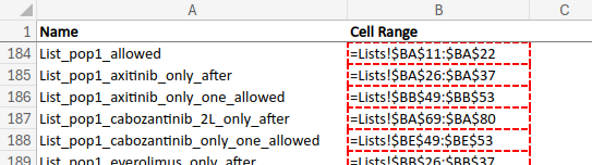
On the named ranges sheet, row 184 has Name List_pop1_allowed and Cell Range =Lists!$BA$11:$BA$22.
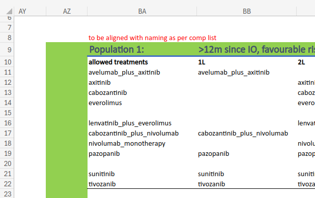
On the Lists sheet, we can see the list of allowed treatments.
Then, if we import the excel spreadsheet, we can view that same parameter within the nested list i.
# Import the functions requiredsource(file.path("../../3_Functions/excel/extract.R"))# Import the excel fileexcel_path <-"../../1_Data/ID6184_RCC_model inputs FAD version [UK RWE unredacted, ACIC redacted, cPAS redacted].xlsm"i <-f_excel_extract(excel_path, verbose =FALSE)# Tidy the imported parametersi <-c(i,f_excel_cleanParams(i$R_table_param))# View the parameteri$List_pop1_allowed
Hazard ratios (HR) from the network meta-analyses (NMA)
PH_NMA_CODA.rds and FPNMA_means.rds
These files contain the outputs of the proportional hazards NMA (PH NMA) and the fractional polynomial NMA (FP NMA). In the publicly available versions, time to next treatment as a surrogate for nivolumab plus ipilimumab is not available to the public as this data was marked as confidential by the data holders.
# Import the NMA resultsRDS_path2 <-"../../1_Data/PH_NMA_CODA.rds"RDS_path3 <-"../../1_Data/FPNMA_means.rds"i$PHNMA <-readRDS(RDS_path2)i$FPNMA$means <-readRDS(RDS_path3)
# Preview the PH NMA resultskable(head(i$PHNMA$data))
run
population
line
molecule
endpoint
referencetreatment
referencetrial
hr
1
0
1
4
0
7
0
0.8958580
1
0
1
1
0
7
0
0.7821468
1
0
1
8
0
7
0
1.4324613
1
0
1
2
0
7
0
0.7571763
1
0
1
5
0
7
0
0.9492596
1
0
1
3
0
7
0
0.8561836
# Preview the FP NMA resultskable(head(i$FPNMA$means))
time
intervention_code
reference_treatment_code
line
endpoint
population
ref_trial_code
V1
0.4615385
4
7
1
1
0
0
6.0866273
0.6923077
4
7
1
1
0
0
0.7948374
0.9230769
4
7
1
1
0
0
0.6307802
1.1538462
4
7
1
1
0
0
0.6127038
1.3846154
4
7
1
1
0
0
0.6141338
1.6153846
4
7
1
1
0
0
0.6184885
In both tables, you can see that each row has a HR (hr/V1), and that these are for each combination of:
The PH NMA results are from a Bayesian analysis and so has lots of samples for each HR (10,000). Hence, the filename is PH_NMA_CODA.rds, with CODA referring to “Convergence Diagnosis and Output Analysis”. When you run a Bayesian analysis, CODA samples are samples from the posterior distribution of your model parameters - in this case, the HRs.
max(i$PHNMA$data$run)
[1] 10000
The FP NMA results are also from a Bayesian analysis, but a mean has been taken of each sample. Hence, the filename FPNMA_means.rds. However, it does have another column time, which is present as FP NMA generates time-varying HR.
Individual patient data (IPD) from the real-world evidence (RWE)
IPD_R_input_noACIC.xlsx
This data represents the results from the RWE study by Challapalli et al. 2022, [1] with the patient-level data from that study shared by the owners of the dataset. In the publicly available version, data has been simulated to replaced data considered confidential by either the UK RWE dataholders or involved companies. The workbook has a sheet IPD which contains the patient-level data we want to import.
# Import data from excelexcel_path2 <-"../../1_Data/IPD_R_input_noACIC.xlsx"wb <-f_excel_extract(excel_path2, verbose =FALSE)# Save to `i` as a data table# (`surv` as will use this data in survival analysis, and `pld` as it is# patient-level data)i$surv$pld <-as.data.table(wb$`_xlnm._FilterDatabase`)# Preview data tablekable(head(i$surv$pld))
This R data file contains the results from a pre-run survival analysis on the patient-level RWE data (i.e. the output of the if statement run if i$dd_run_surv_reg == "Yes" in Model_Structure.R). In the publicly available version, time to discontinuation (TTD) and time to progression (TTP) are set equal to PFS in order to protect data considered confidential by the involved companies, and post-progression survival (PPS) is set equal to the UK RWE
The R data file is a large nested list from which you can select a:
Challapalli A, Ratnayake G, McGrane J, Frazer R, Gupta S, Parslow DS, et al. 1463PPatterns of care and outcomes of metastatic renal cell carcinoma (mRCC) patients (pts) with bone metastases (BM): AUK multicenter review. Annals of Oncology 2022;33:S1215. https://doi.org/10.1016/j.annonc.2022.07.1566.