# To run model
import PHC

# To import results and produce figures
from reproduction_helpers import process_results
import pandas as pd
import os
import matplotlib.pyplot as plt
import matplotlib.ticker as ticker
import itertools

# To speed up run time
from multiprocessing import Pool

# Additional package to record runtime of this notebook
import time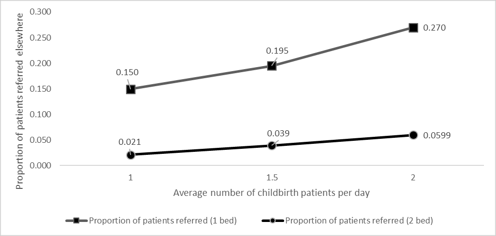
start = time.time()Reproducing Figure 4
This notebook aims to reproduce Figure 4 from Shoaib M, Ramamohan V. Simulation modeling and analysis of primary health center operations. SIMULATION 98(3):183-208. (2022). https://doi.org/10.1177/00375497211030931.
Parameters
In this figure, we vary configuration 1 as follows:
- Number of delivery beds: 2 or 3
- Delivery arrivals: 1, 1.5 or 2 per day
- 1 = IAT 1440 (as in e.g. config1)
- 1.5 = 960 (as 720+240=960, and 960+480=1440)
- 2 = IAT 720 (as we did for Figure 3)
Set up
# Paths to save image files to
output_folder = '../outputs'
fig4_path = os.path.join(output_folder, 'fig4.png')
Run model
# Varying number of childbirth cases
arr_dict = [
    {
        'delivery_iat': 1440,
        'rep_file': 'arr1440'
    },
    {
        'delivery_iat': 1080,
        'rep_file': 'arr1080'
    },
    {
        'delivery_iat': 960,
        'rep_file': 'arr960'
    },
    {
        'delivery_iat': 720,
        'rep_file': 'arr720'
    }
]

# Varying the number of beds
bed_dict = [
    {
        'delivery_bed_n': 1,
        'rep_file': 'bed1'
    },
    {
        'delivery_bed_n': 2,
        'rep_file': 'bed2'
    }
]
Create each combination for the reproduction
dict_list = []
for arr in arr_dict:
    for bed in bed_dict:
        # Combine the dictionaries
        comb = {**arr, **bed}
        # Replace the file name
        comb['rep_file'] = f'''f4_{arr['rep_file']}_{bed['rep_file']}.xls'''
        # Save to list
        dict_list.append(comb)

len(dict_list)8# Append 's_' to all items
for i, d in enumerate(dict_list):
dict_list[i] = {f's_{k}': v for k, v in d.items()}
# Preview example
dict_list[0]{'s_delivery_iat': 1440,
's_rep_file': 'f4_arr1440_bed1.xls',
's_delivery_bed_n': 1}Run the model (with parallel processing to reduce run time)
# Wrapper function to allow input of dictionary with pool
def wrapper(d):
    return PHC.main(**d)

# Create a process pool that uses all CPUs
with Pool(8) as pool:
    # Run PHC.main() using each of inputs from config
    pool.map(wrapper, dict_list)
No of replications done No of replications done 00
No of replications done 0
No of replications done 0
No of replications done 0
No of replications done 0
No of replications done 0
No of replications done 0
No of replications done 1
No of replications done 1
No of replications done 1
No of replications done 1
No of replications done 1
No of replications done 1
No of replications done 1
No of replications done 2
No of replications done 2
No of replications done 2
No of replications done 2
No of replications done 2
No of replications done 1
No of replications done 2
No of replications done 2
No of replications done 3
No of replications done 3
No of replications done 3
No of replications done 3
No of replications done 3
No of replications done 2
No of replications done 3
No of replications done 4
No of replications done 4
No of replications done 4
No of replications done 4
No of replications done 3
No of replications done 3
No of replications done 4
No of replications done 4
No of replications done 5
No of replications done 5
No of replications done 5
No of replications done 5
No of replications done 4
No of replications done 5
No of replications done 4
No of replications done 6
No of replications done 6
No of replications done 6
No of replications done 6
No of replications done 5
No of replications done 5
No of replications done 6
No of replications done 7
No of replications done 7
No of replications done 7
No of replications done 7
No of replications done 5
No of replications done 6
No of replications done 7
No of replications done 6
No of replications done 8
No of replications done 8
No of replications done 8
No of replications done 8
No of replications done 6
No of replications done 7
No of replications done 8
No of replications done 9
No of replications done 9
No of replications done 9
No of replications done 7
No of replications done 9
No of replications done 7
No of replications done 8
No of replications done 9
No of replications done 8
No of replications done 8
No of replications done 9
No of replications done 9
No of replications done 9Process results
data = process_results([i['s_rep_file'] for i in dict_list], xls=True)
data.head()| f4_arr1440_bed1 | f4_arr1440_bed2 | f4_arr1080_bed1 | f4_arr1080_bed2 | f4_arr960_bed1 | f4_arr960_bed2 | f4_arr720_bed1 | f4_arr720_bed2 | |
|---|---|---|---|---|---|---|---|---|
| OPD patients | 33101.900000 | 33194.200000 | 33169.20000 | 33202.900000 | 33085.500000 | 33191.200000 | 33067.70000 | 33071.400000 |
| IPD patients | 184.800000 | 182.600000 | 183.30000 | 183.600000 | 189.600000 | 185.300000 | 184.70000 | 179.900000 |
| ANC patients | 359.300000 | 360.600000 | 369.80000 | 364.700000 | 359.900000 | 367.300000 | 363.00000 | 361.700000 |
| Del patients | 353.800000 | 361.400000 | 480.70000 | 494.400000 | 556.100000 | 552.800000 | 728.90000 | 731.100000 |
| OPD Q wt | 0.008353 | 0.008172 | 0.01205 | 0.012351 | 0.011181 | 0.014176 | 0.01906 | 0.018819 |
Create Figure 4
# Select series with proportion referred
a4 = data.loc['prop_del_referred']

# Reshape into appropriate format for plotting
names = ['1 (IAT 1440)', '1.5 (IAT 960)', '1.5 (IAT1080)', '2 (IAT 720)']
bed1 = [a4['f4_arr1440_bed1'], a4['f4_arr960_bed1'],
        a4['f4_arr1080_bed1'], a4['f4_arr720_bed1']]
bed2 = [a4['f4_arr1440_bed2'], a4['f4_arr960_bed2'],
        a4['f4_arr1080_bed2'], a4['f4_arr720_bed2']]

data_4a = pd.DataFrame({'1 bed': bed1, '2 beds': bed2}, index=names)
data_4a| 1 bed | 2 beds | |
|---|---|---|
| 1 (IAT 1440) | 0.147775 | 0.017549 |
| 1.5 (IAT 960) | 0.225166 | 0.037351 |
| 1.5 (IAT1080) | 0.185273 | 0.033162 |
| 2 (IAT 720) | 0.273051 | 0.057273 |
Function to create figure
def create_figure4(df):
    '''
    Produces figure 4
    '''
    # Plot data
    ax = df.plot(kind='line', color='black')

    # Add markers
    for l, ms in zip(ax.lines, itertools.cycle('so')):
        l.set_marker(ms)
        l.set_color('black')
    ax.legend(title='Number of delivery beds')

    # Add labels to each point
    for line in ax.lines:
        x_data = line.get_xdata()
        y_data = line.get_ydata()
        for x, y in zip(x_data, y_data):
            ax.annotate(f'{y:.3f}', xy=(x, y), xytext=(3, 3),
                        textcoords='offset points', fontsize=9)

    # Adjust figure
    plt.xlabel('Average number of childbirth patients per day')
    plt.ylabel('Proportion of patients referred elsewhere')
    plt.ylim(0, 0.3)
    ax.xaxis.set_major_locator(ticker.MultipleLocator(1))
    plt.grid(axis='y')
    ax.set_axisbelow(True)
Evaluating options
Due to discrepancies observed for 1.5 arrivals, I presumed that the difference could be in the IAT used, since the paper only provides the number of arrivals and not the IAT. I estimated the IAT to be 960, but I also tried using 1080 (which is equidistant between the 1 and 2 arrival IAT values), as I have not identified a formula for how these are produced, and have only been able to estimate.
From comparing the two options, 960 is closer for 2 beds whilst 1080 is closer for 1 bed. Since the difference is greatest for 1 bed, I opted to use that IAT.
create_figure4(data_4a)
# plt.savefig(fig4_path, bbox_inches='tight')
plt.show()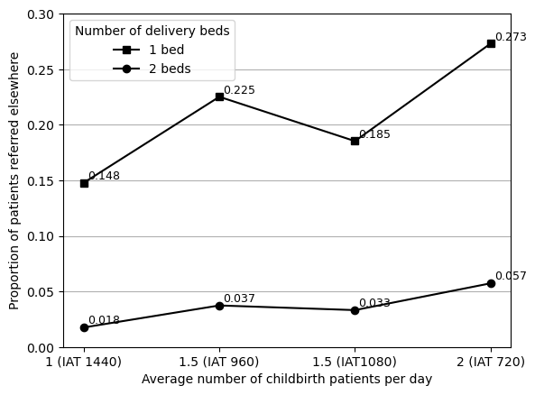
# Input results from original and reproduced figures
comp = pd.DataFrame({
    'original': [0.021, 0.039, 0.039, 0.0599, 0.150, 0.195, 0.195, 0.270],
    'reproduced': data_4a.iloc[:, 1].to_list() + data_4a.iloc[:, 0].to_list()})
comp['reproduced'] = round(comp['reproduced'], 3)

# Find size of difference and % change
comp['diff'] = comp['reproduced'] - comp['original']
comp['pct_change'] = comp.pct_change(axis=1).iloc[:, 1]*100
comp| original | reproduced | diff | pct_change | |
|---|---|---|---|---|
| 0 | 0.0210 | 0.018 | -0.0030 | -14.285714 |
| 1 | 0.0390 | 0.037 | -0.0020 | -5.128205 |
| 2 | 0.0390 | 0.033 | -0.0060 | -15.384615 |
| 3 | 0.0599 | 0.057 | -0.0029 | -4.841402 |
| 4 | 0.1500 | 0.148 | -0.0020 | -1.333333 |
| 5 | 0.1950 | 0.225 | 0.0300 | 15.384615 |
| 6 | 0.1950 | 0.185 | -0.0100 | -5.128205 |
| 7 | 0.2700 | 0.273 | 0.0030 | 1.111111 |
Chosen figure (with IAT 1080)
# Drop 960
data_4a_final = data_4a.drop(index='1.5 (IAT 960)')

# Amend labels to match original
data_4a_final.index = [x.split(' (')[0] for x in data_4a_final.index.to_list()]

create_figure4(data_4a_final)
plt.savefig(fig4_path, bbox_inches='tight')
plt.show()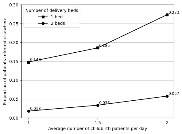
Run time
# Find run time in seconds
end = time.time()
runtime = round(end-start)

# Display converted to minutes and seconds
print(f'Notebook run time: {runtime//60}m {runtime%60}s')
Notebook run time: 3m 0s