# To run model
import PHC

# To import results and produce figures
from reproduction_helpers import process_results
import pandas as pd
import os
import matplotlib.pyplot as plt
import numpy as np

# To speed up run time
from multiprocessing import Pool

# Additional package to record runtime of this notebook
import time
start = time.time()Reproducing Figure 3A-D and in-text result 1
This notebook aims to reproduce Figures 3A-D and in-text result 1 from Shoaib M, Ramamohan V. Simulation modeling and analysis of primary health center operations. SIMULATION 98(3):183-208. (2022). https://doi.org/10.1177/00375497211030931.
In-text result 1:
“We also note that waiting times for outpatient-related resources (laboratory, OPD consultation, etc. - not depicted in Figures 3a – 3d) increase marginally because the associated resources are also required by inpatient/childbirth/ANC cases, which increase in number in the above scenarios”
Parameters
In these figures, we vary configuration 1 as follows:
- Number of inpatient/childbirth/ANC cases per day:
- 1 = IAT 1440 (e.g. like IPD cases for config1)
- 2 = IAT 720 (as 2880 is 0.5 per day and 1440 is 1 per day)
- Average service time for outpatients:
- 0.87 (0.21) (same as config1)
- 2.5 (0.5) (as in figure 2)
Set up
# Paths to save image files to
output_folder = '../outputs'
fig3a_path = os.path.join(output_folder, 'fig3a.png')
fig3b_path = os.path.join(output_folder, 'fig3b.png')
fig3c_path = os.path.join(output_folder, 'fig3c.png')
fig3d_path = os.path.join(output_folder, 'fig3d.png')
txt1_path = os.path.join(output_folder, 'intext1.csv')
Run model
# Varying number of inpatient, childbirth and ANC cases
arr_dict = [
    {
        'IPD_iat': 1440,
        'delivery_iat': 1440,
        'ANC_iat': 1440,
        'rep_file': 'arr111'
    },
    {
        'IPD_iat': 720,
        'delivery_iat': 1440,
        'ANC_iat': 1440,
        'rep_file': 'arr211',
    },
    {
        'IPD_iat': 720,
        'delivery_iat': 720,
        'ANC_iat': 720,
        'rep_file': 'arr222',
    }
]

# Varying service time
serv_dict = [
    {
        'mean': 0.87,
        'sd': 0.21,
        'consult_boundary_1': 0.5,  # From PHC.py
        'consult_boundary_2': 0.3,  # From PHC.py
        'rep_file': 'serv087'
    },
    {
        'mean': 2.5,
        'sd': 0.5,
        'consult_boundary_1': 1,  # From Figure 2 (which was a guess)
        'consult_boundary_2': 1,  # From Figure 2 (which was a guess)
        'rep_file': 'serv25'
    }
]
Create each combination for the reproduction
dict_list = []
for arr in arr_dict:
    for serv in serv_dict:
        # Combine the dictionaries
        comb = {**arr, **serv}
        # Replace the file name
        comb['rep_file'] = f'''f3_{arr['rep_file']}_{serv['rep_file']}.xls'''
        # Save to list
        dict_list.append(comb)

len(dict_list)6# Append 's_' to all items
for i, d in enumerate(dict_list):
dict_list[i] = {f's_{k}': v for k, v in d.items()}
# Preview example
dict_list[0]{'s_IPD_iat': 1440,
's_delivery_iat': 1440,
's_ANC_iat': 1440,
's_rep_file': 'f3_arr111_serv087.xls',
's_mean': 0.87,
's_sd': 0.21,
's_consult_boundary_1': 0.5,
's_consult_boundary_2': 0.3}Run the model (with parallel processing to reduce run time)
# Wrapper function to allow input of dictionary with pool
def wrapper(d):
    return PHC.main(**d)

# Create a process pool that uses all CPUs
with Pool() as pool:
    # Run PHC.main() using each of inputs from config
    pool.map(wrapper, dict_list)
No of replications done 0
No of replications done 0
No of replications done 0
No of replications done 0
No of replications done 0
No of replications done 0
No of replications done 1
No of replications done 1
No of replications done 1
No of replications done 1
No of replications done 1
No of replications done 1
No of replications done 2
No of replications done 2
No of replications done 2
No of replications done 2
No of replications done 2
No of replications done 2
No of replications done 3
No of replications done 3
No of replications done 3
No of replications done 3
No of replications done 3
No of replications done 3
No of replications done 4
No of replications done 4
No of replications done 4
No of replications done 4
No of replications done 4
No of replications done 4
No of replications done 5
No of replications done 5
No of replications done 5
No of replications done 5
No of replications done 5
No of replications done 5
No of replications done 6
No of replications done 6
No of replications done 6
No of replications done 6
No of replications done 6
No of replications done 7
No of replications done 7
No of replications done 6
No of replications done 7
No of replications done 7
No of replications done 8
No of replications done 8
No of replications done 8
No of replications done 7
No of replications done 8
No of replications done 7
No of replications done 9
No of replications done 9
No of replications done 9
No of replications done 9
No of replications done 8
No of replications done 8
No of replications done 9
No of replications done 9Process results
Function for reshaping these as repeat a few times
def reshape_087_25(s):
    '''
    Reshapes series that has results from scenarios including mean 0.87 and 2.5
    to produce a 3 x 2 dataframe where rows are consultation time and columns
    are the arrivals

    Parameters:
    -----------
    s : series
        Series with results from figure 3 model variants

    Returns:
    --------
    res : dataframe
        Dataframe where rows are consultation time and columns are arrivals
    '''
    # Reshape data so in appropriate format for plotting grouped bar chart
    names = ['0.87 (0.21)', '2.5 (0.5)']
    s111 = [s['f3_arr111_serv087'], s['f3_arr111_serv25']]
    s211 = [s['f3_arr211_serv087'], s['f3_arr211_serv25']]
    s222 = [s['f3_arr222_serv087'], s['f3_arr222_serv25']]

    res = pd.DataFrame(
        {'(1/1/1)': s111, '(2/1/1)': s211, '(2/2/2)': s222}, index=names)

    return res
def plot_087_25(df, ylab, ylim=False, save_path=False):
'''
Plots results from varying cases and consultation time
Parameters:
-----------
df : pd.DataFrame
Dataframe reshaped using reshape_087_25()
'''
# Plot data
ax = df.plot.bar(edgecolor='black', color='white', width=0.7)
# Add patterns
bars = ax.patches
pattern = np.repeat(['++', '\\\\\\\\', '//////'], 2)
for bar, hatch in zip(bars, pattern):
bar.set_hatch(hatch)
ax.legend(title='Inpatient/Childbirth/ANC cases per day')
# Adjust figure
plt.xlabel('Consultation time (minutes): mean (SD)')
plt.ylabel(ylab)
plt.xticks(rotation=0)
ax.grid(axis='y')
if ylim:
plt.ylim(ylim)
ax.set_axisbelow(True)
if save_path:
plt.savefig(save_path, bbox_inches='tight')
plt.show()Create Figure 3A
# Import and process results
data_full = process_results([
'f3_arr111_serv087', 'f3_arr211_serv087', 'f3_arr222_serv087',
'f3_arr111_serv25', 'f3_arr211_serv25', 'f3_arr222_serv25'])
# Filter to doctor utilisation
a3 = data_full.loc['doc occ']
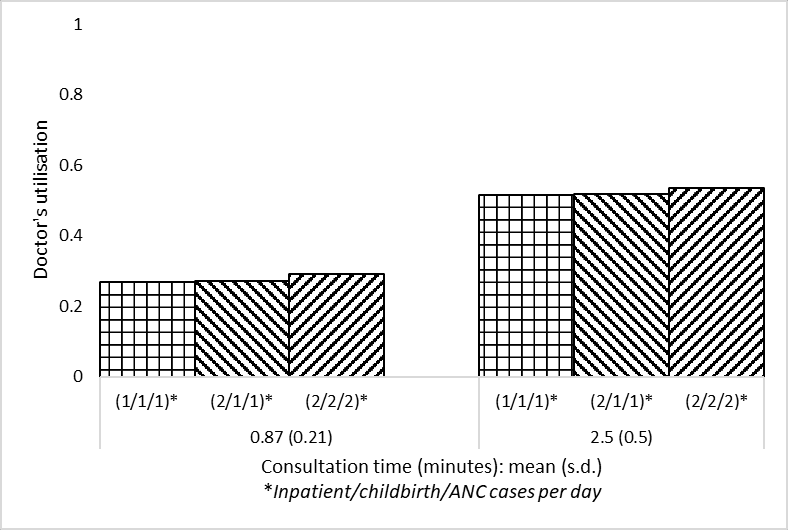
a3f3_arr111_serv087 0.269200
f3_arr211_serv087 0.270328
f3_arr222_serv087 0.289834
f3_arr111_serv25 0.513831
f3_arr211_serv25 0.517641
f3_arr222_serv25 0.537557
Name: doc occ, dtype: float64# Reshape data so in appropriate format for plotting grouped bar chart
data_3a = reshape_087_25(a3)
data_3a| (1/1/1) | (2/1/1) | (2/2/2) | |
|---|---|---|---|
| 0.87 (0.21) | 0.269200 | 0.270328 | 0.289834 |
| 2.5 (0.5) | 0.513831 | 0.517641 | 0.537557 |
plot_087_25(data_3a, ylab='''Doctor's utilisation''',
            ylim=[0,1], save_path=fig3a_path)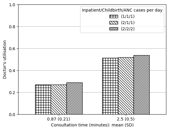
Creating Figure 3B
# Filter to staff nurse utilisation and config1 (0.87)
data_3b = data_full.loc[
'staff nurse occ', data_full.columns.str.endswith('087')]
# Rename index
data_3b = data_3b.rename(index={'f3_arr111_serv087': '(1/1/1)',
'f3_arr211_serv087': '(2/1/1)',
'f3_arr222_serv087': '(2/2/2)'})
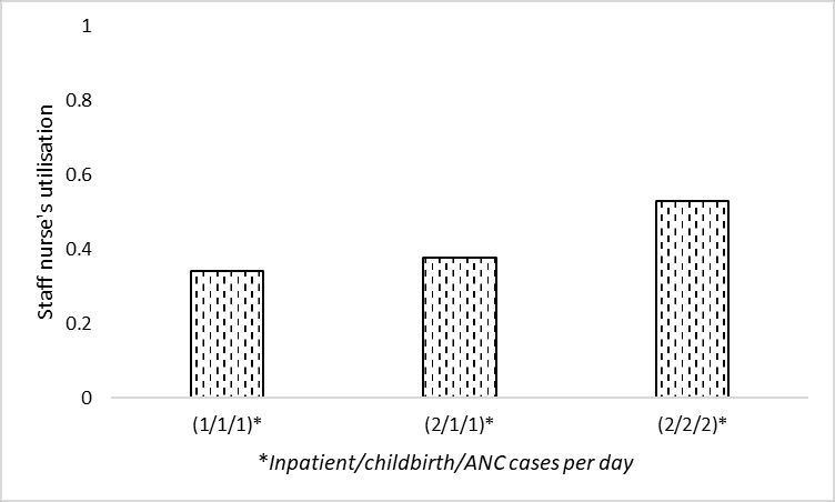
data_3b(1/1/1) 0.343989
(2/1/1) 0.378359
(2/2/2) 0.532546
Name: staff nurse occ, dtype: float64ax = data_3b.plot.bar(edgecolor='black', color='white', hatch='..')
plt.xlabel('Inpatient/childbirth/ANC cases per day')
plt.ylabel('''Staff nurse's utilisation''')
plt.ylim(0, 1)
plt.xticks(rotation=0)
ax.grid(axis='y')
ax.set_axisbelow(True)
plt.savefig(fig3b_path, bbox_inches='tight')
plt.show()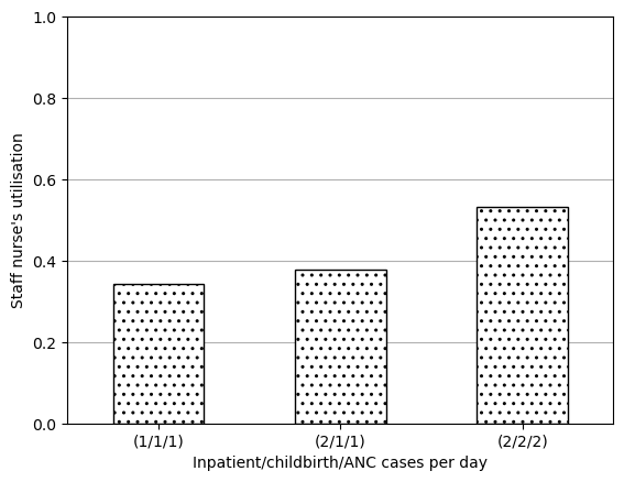
Creating Figure 3C
# Filter to inpatient bed utilisation and config1 (0.87)
data_3c = data_full.loc[
'ipd bed occ', data_full.columns.str.endswith('087')]
# Rename index
data_3c = data_3c.rename(index={'f3_arr111_serv087': '(1/1/1)',
'f3_arr211_serv087': '(2/1/1)',
'f3_arr222_serv087': '(2/2/2)'})
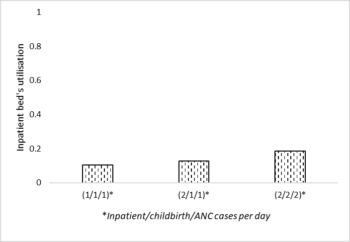
data_3c(1/1/1) 0.107832
(2/1/1) 0.129961
(2/2/2) 0.186271
Name: ipd bed occ, dtype: float64ax = data_3c.plot.bar(edgecolor='black', color='white', hatch='..')
plt.xlabel('Inpatient/childbirth/ANC cases per day')
plt.ylabel('Inpatient bed utilisation')
plt.ylim(0, 1)
plt.xticks(rotation=0)
ax.grid(axis='y')
ax.set_axisbelow(True)
plt.savefig(fig3c_path, bbox_inches='tight')
plt.show()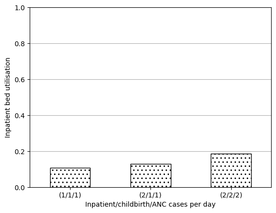
Creating Figure 3D
# Filter to proportion of childbirth cases referred and config1 (0.87)
data_3d = data_full.loc[
'prop_del_referred', data_full.columns.str.endswith('087')]
# Rename index
data_3d = data_3d.rename(index={'f3_arr111_serv087': '(1/1/1)',
'f3_arr211_serv087': '(2/1/1)',
'f3_arr222_serv087': '(2/2/2)'})
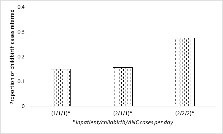
data_3d(1/1/1) 0.151000
(2/1/1) 0.143832
(2/2/2) 0.271968
Name: prop_del_referred, dtype: float64ax = data_3d.plot.bar(edgecolor='black', color='white', hatch='..')
plt.xlabel('Inpatient/childbirth/ANC cases per day')
plt.ylabel('Proportion of childbirth cases referred')
plt.yticks(np.arange(0, 0.5, 0.1))
plt.xticks(rotation=0)
ax.grid(axis='y')
ax.set_axisbelow(True)
plt.savefig(fig3d_path, bbox_inches='tight')
plt.show()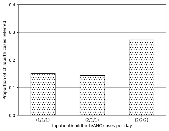
Reproducing in-text result 1
This result refers to “waiting times for outpatient-related resources (laboratory, OPD consultation, etc.)”. I assume this to refer to:
- OPD queue waiting time (minutes)
- Lab queue waiting time (minutes)
# Get OPD queue time
data_txt1_opd = reshape_087_25(data_full.loc['OPD Q wt'])
data_txt1_opd['Output'] = 'OPD queue waiting time (minutes)'

# Get lab queue time
data_txt1_lab = reshape_087_25(data_full.loc['Lab Q wt'])
data_txt1_lab['Output'] = 'Lab queue waiting time (minutes)'

# Combine, round, save and show dataframe
data_txt1 = round(pd.concat([data_txt1_opd, data_txt1_lab]), 3)
data_txt1.index.names = ['Consultation time: mean (SD)']
data_txt1.to_csv(txt1_path)
data_txt1| (1/1/1) | (2/1/1) | (2/2/2) | Output | |
|---|---|---|---|---|
| Consultation time: mean (SD) | ||||
| 0.87 (0.21) | 0.011 | 0.010 | 0.023 | OPD queue waiting time (minutes) |
| 2.5 (0.5) | 0.121 | 0.124 | 0.158 | OPD queue waiting time (minutes) |
| 0.87 (0.21) | 2.069 | 2.070 | 2.110 | Lab queue waiting time (minutes) |
| 2.5 (0.5) | 2.314 | 2.322 | 2.308 | Lab queue waiting time (minutes) |
Produced figures but, due to the very small amount of change observed in minutes, feel it is misleading, so will just save table.
plot_087_25(data_txt1_opd, ylab='OPD queue waiting time (minutes)')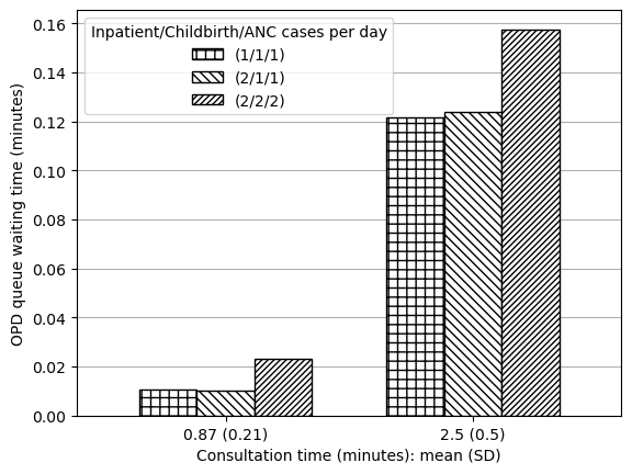
plot_087_25(data_txt1_lab, ylim=[0, 3], ylab='Lab queue waiting time (minutes)')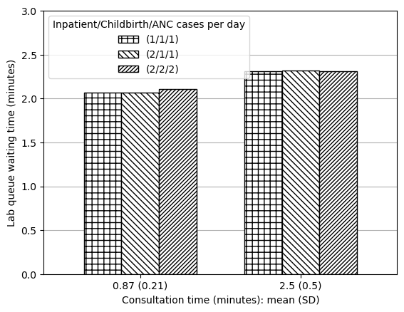
Run time
# Find run time in seconds
end = time.time()
runtime = round(end-start)

# Display converted to minutes and seconds
print(f'Notebook run time: {runtime//60}m {runtime%60}s')
Notebook run time: 2m 45s