Reproduce Figures 2-4 and in-text results 1-3

The majority of the items in the model scope are reproduced in this file, but Figure 5 and the supplementary figure are created in seperate .qmd files.

This decision was primarily due to issues with RStudio crashing when running all scenarios from a single .Rmd file.

Run time: 18.024 minutes (will vary between machines)

Set up

# Clear environment
rm(list=ls())

# Start timer
start.time <- Sys.time()

# Disable scientific notation
options(scipen=999)

# Import required libraries (if not otherwise import in R scripts below)
library(ggpubr)

Loading required package: ggplot2

library(tidyr, include.only = c("pivot_wider"))

# Get the model and helper functions (but hide loading warnings for each package)
suppressMessages(source("model.R"))
suppressMessages(source("helpers.R"))

# Set the seed and default dimensions for figures
SEED = 200
DEFAULT_WIDTH = 7
DEFAULT_HEIGHT = 4

# Set file paths to save results

folder = "../outputs"

path_baseline_f2 <- file.path(folder, "fig2_baseline.csv.gz")
path_exclusive_f2 <- file.path(folder, "fig2_exclusive.csv.gz")
path_twoangio_f2 <- file.path(folder, "fig2_twoangio.csv.gz")

path_baseline_f3 <- file.path(folder, "fig3_baseline.csv.gz")
path_exclusive_f3 <- file.path(folder, "fig3_exclusive.csv.gz")
path_twoangio_f3 <- file.path(folder, "fig3_twoangio.csv.gz")

path_txt2 <- file.path(folder, "txt2.csv") # Used for results 1 and 2
path_txt3 <- file.path(folder, "txt3.csv")
path_fig2 <- file.path(folder, "fig2.png")
path_fig3 <- file.path(folder, "fig3.png")
path_fig4 <- file.path(folder, "fig4.png")

Run models

Set to true or false, depending on whether you want to run everything.

run <- FALSE

Run model scenarios.

if (isTRUE(run)) {
  # Run model
  baseline <- run_model(seed = SEED)
  baseline_6pm <- run_model(shifts = c(8,18), seed = SEED)
  baseline_7pm <- run_model(shifts = c(8,19), seed = SEED)

  exclusive <- run_model(exclusive_use = TRUE, seed = SEED)
  exclusive_6pm <- run_model(shifts = c(8,18), exclusive_use = TRUE, seed = SEED)
  exclusive_7pm <- run_model(shifts = c(8,19), exclusive_use = TRUE, seed = SEED)

  twoangio <- run_model(angio_inr = 2, angio_ir=0, seed = SEED)
  twoangio_6pm <- run_model(shifts = c(8,18), angio_inr = 2, angio_ir=0, seed = SEED)
  twoangio_7pm <- run_model(shifts = c(8,19), angio_inr = 2, angio_ir=0, seed = SEED)
}

# (in seperate cell to above as otherwise seemed to crash)
if (isTRUE(run)) {
  # Save results for Figure 2
  data.table::fwrite(baseline, path_baseline_f2)
  data.table::fwrite(exclusive, path_exclusive_f2)
  data.table::fwrite(twoangio, path_twoangio_f2)

  # Process and save results for Figure 3
  process_f3_data(baseline, baseline_6pm, baseline_7pm, path_baseline_f3)
  process_f3_data(exclusive, exclusive_6pm, exclusive_7pm, path_exclusive_f3)
  process_f3_data(twoangio, twoangio_6pm, twoangio_7pm, path_twoangio_f3)

  # Remove the dataframes from environment
  rm(baseline, baseline_6pm, baseline_7pm,
     exclusive, exclusive_6pm, exclusive_7pm,
     twoangio, twoangio_6pm, twoangio_7pm)
}

Import results

Import the results, adding a column to each to indicate the scenario.

base_f2 <- import_results(path_baseline_f2,
                          "Baseline")
exc_f2 <- import_results(path_exclusive_f2,
                         "Exclusive use")
two_f2 <- import_results(path_twoangio_f2,
                         "Two AngioINRs")

base_f3 <- import_results(path_baseline_f3,
                          "Baseline")
exc_f3 <- import_results(path_exclusive_f3,
                         "Exclusive use")
two_f3 <- import_results(path_twoangio_f3,
                         "Two AngioINRs")

In-text results

In-text results 1 and 2

txt2 <- dplyr::bind_rows(base_f2, exc_f2, two_f2) %>%
  filter(resource=="angio_inr") %>%
  group_by(scenario) %>%
  summarize(mean = mean(wait_time)) %>%
  mutate(diff_from_baseline = round(mean - mean[1], 2))

# Save and display result
data.table::fwrite(txt2, path_txt2)
txt2

# A tibble: 3 × 3
  scenario       mean diff_from_baseline
  <chr>         <dbl>              <dbl>
1 Baseline      14.0                0   
2 Exclusive use  8.12              -5.84
3 Two AngioINRs  9.62              -4.34

In-text result 3

txt3 <- dplyr::bind_rows(base_f3, exc_f3, two_f3) %>%
  filter(resource=="angio_inr") %>%
  group_by(scenario, shift) %>%
  summarize(mean = mean(wait_time)) %>%
  mutate(diff_from_5pm = round(mean - mean[1], 2))

`summarise()` has grouped output by 'scenario'. You can override using the
`.groups` argument.

# Save and display result
data.table::fwrite(txt3, path_txt3)
txt3

# A tibble: 9 × 4
# Groups:   scenario [3]
  scenario      shift  mean diff_from_5pm
  <chr>         <chr> <dbl>         <dbl>
1 Baseline      5pm   14.0           0   
2 Baseline      6pm   12.5          -1.47
3 Baseline      7pm   12.5          -1.47
4 Exclusive use 5pm    8.12          0   
5 Exclusive use 6pm    7.80         -0.31
6 Exclusive use 7pm    6.43         -1.69
7 Two AngioINRs 5pm    9.62          0   
8 Two AngioINRs 6pm    9.22         -0.4 
9 Two AngioINRs 7pm    8.70         -0.92

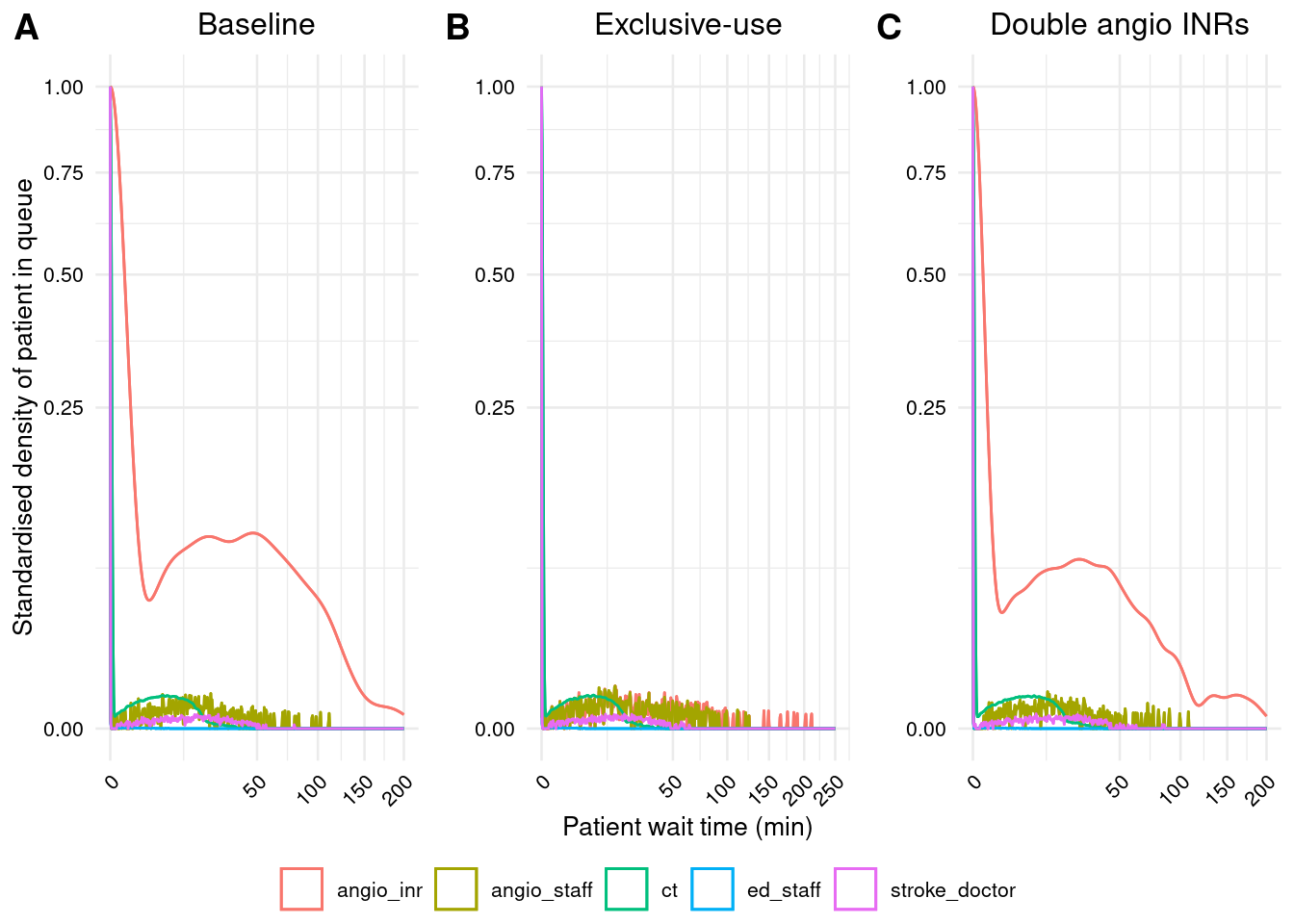
Figure 2

# Create sub-plots
p1 <- create_plot(base_f2,
                  group="resource",
                  title="Baseline",
                  ylab="Standardised density of patient in queue")
p2 <- create_plot(exc_f2,
                  group="resource",
                  title="Exclusive-use",
                  xlab="Patient wait time (min)",
                  xlim=c(0, 250))
p3 <- create_plot(two_f2,
                  group="resource",
                  title="Double angio INRs")

# Arrange in a single figure
ggarrange(p1, p2, p3, nrow=1,
          common.legend=TRUE, legend="bottom",
          labels=c("A", "B", "C"))

Warning: Removed 1 row containing non-finite outside the scale range (`stat_density()`).
Removed 1 row containing non-finite outside the scale range (`stat_density()`).
Removed 1 row containing non-finite outside the scale range (`stat_density()`).
Removed 1 row containing non-finite outside the scale range (`stat_density()`).
Removed 1 row containing non-finite outside the scale range (`stat_density()`).
Removed 1 row containing non-finite outside the scale range (`stat_density()`).
Removed 1 row containing non-finite outside the scale range (`stat_density()`).
Removed 1 row containing non-finite outside the scale range (`stat_density()`).

ggsave(path_fig2, width=DEFAULT_WIDTH, height=DEFAULT_HEIGHT)

Demonstrate that geom_density scaled is scaling against density of 0 wait time

# Create figure as usual
p <- create_plot(base_f2,
                 group="resource",
                 title="Baseline",
                 ylab="Standardised density of patient in queue")

# Get data from the plot
plot_data <- ggplot_build(p)$data[[1]]

Warning: Removed 1 row containing non-finite outside the scale range (`stat_density()`).
Removed 1 row containing non-finite outside the scale range (`stat_density()`).

# Create dataframe with the densities for when the waitimes are 0
no_wait <- plot_data %>% filter(x==0) %>% select(colour, density, scaled)

# Loop through each of the colours (which reflect the resource groups)
for (c in no_wait$colour) {
  # Filter the plot data to that resource group, then divide the densities by
  # the density from wait time 0
  d <- plot_data %>%
    filter(colour == c) %>%
    mutate(scaled2 = density / no_wait[no_wait$colour==c, "density"]) %>%
    ungroup() %>%
    select(scaled, scaled2)

  # Find the number of rows where these values match the scaled values
  n_match <- sum(apply(d, 1, function(x) length(unique(x)) == 1))
  n_total <- nrow(d)
  print(sprintf("%s out of %s results match", n_match, n_total))
}

[1] "512 out of 512 results match"
[1] "512 out of 512 results match"
[1] "512 out of 512 results match"
[1] "512 out of 512 results match"
[1] "512 out of 512 results match"

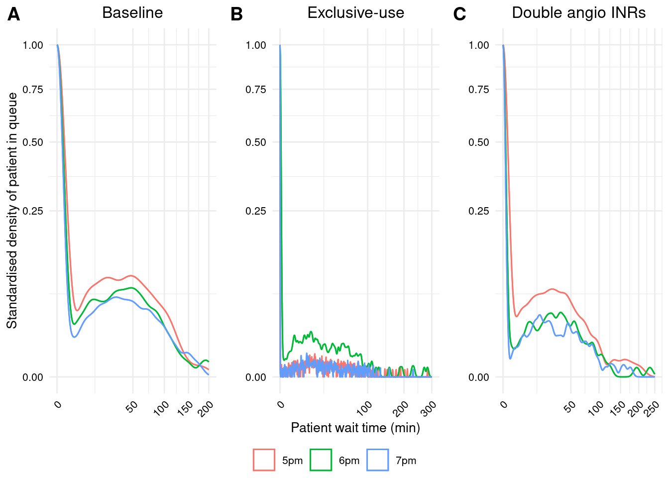
Figure 3

# Create sub-plots
p1 <- create_plot(base_f3,
                  group="shift",
                  title="Baseline",
                  ylab="Standardised density of patient in queue")
p2 <- create_plot(exc_f3,
                  group="shift",
                  title="Exclusive-use",
                  xlab="Patient wait time (min)",
                  xlim=c(0, 300),
                  breaks_width=100)
p3 <- create_plot(two_f3,
                  group="shift",
                  title="Double angio INRs",
                  xlim=c(0, 250))

# Arrange in a single figure
ggarrange(p1, p2, p3, nrow=1,
          common.legend=TRUE, legend="bottom",
          labels=c("A", "B", "C"))

Warning: Removed 5 rows containing non-finite outside the scale range
(`stat_density()`).
Removed 5 rows containing non-finite outside the scale range
(`stat_density()`).
Removed 5 rows containing non-finite outside the scale range
(`stat_density()`).
Removed 5 rows containing non-finite outside the scale range
(`stat_density()`).

Warning: Removed 1 row containing non-finite outside the scale range (`stat_density()`).
Removed 1 row containing non-finite outside the scale range (`stat_density()`).

Warning: Removed 2 rows containing non-finite outside the scale range
(`stat_density()`).
Removed 2 rows containing non-finite outside the scale range
(`stat_density()`).

ggsave(path_fig3, width=DEFAULT_WIDTH, height=DEFAULT_HEIGHT)

Figure 4

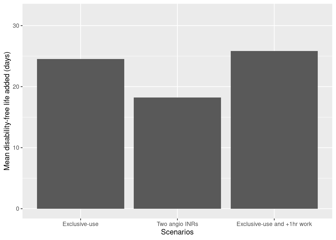
# Get the relevant results from in-text results 1, 2 and 3
# Then calculate difference from baseline
fig4 <- dplyr::bind_rows(txt2 %>% select(scenario, mean),
                         txt3 %>%
                          filter(scenario=="Exclusive use", shift=="6pm") %>%
                          mutate(scenario="Exclusive use (+1h)") %>%
                          select(scenario, mean)) %>%
  mutate(diff = mean - mean[1]) %>%
  filter(scenario!="Baseline") %>%
  mutate(dis_free_gain = abs(diff)*4.2)

# Set order of the bars, and give full labels
fig4_col <- c("Exclusive use", "Two AngioINRs", "Exclusive use (+1h)")
fig4_col_l <- c("Exclusive-use", "Two angio INRs", "Exclusive-use and +1hr work")
fig4$scenario <- factor(fig4$scenario, levels=fig4_col)
fig4$scenario_lab <- plyr::mapvalues(fig4$scenario, from=fig4_col, to=fig4_col_l)

ggplot(fig4, aes(x=scenario_lab, y=dis_free_gain)) +
  geom_bar(stat="identity") +
  ylim(0, 32) +
  xlab("Scenarios") +
  ylab("Mean disability-free life added (days)")

ggsave(path_fig4, width=5, height=3)

Time elapsed

if (isTRUE(run)) {
  end.time <- Sys.time()
  elapsed.time <- round((end.time - start.time), 3)
  elapsed.time
}