Learning objectives:
- Understand the importance of being able to run all your analysis from start to end with a single command.
- Learn about options for executing multiple scripts/files in order.
- Know how to write and use bash scripts for this purpose.
- Explore opportunities with literate programming.
Relevant reproducibility guidelines:
- STARS Reproducibility Recommendations (⭐): Ensure model parameters are correct.
- NHS Levels of RAP (🥈): Outputs are produced by code with minimal manual intervention.
Pipeline: running from start to end
As introduced at the start of this book, a reproducible analytical pipeline (RAP) is a systematic approach to data analysis and modelling in which every step of the process (end-to-end) is transparent, automated, and repeatable.
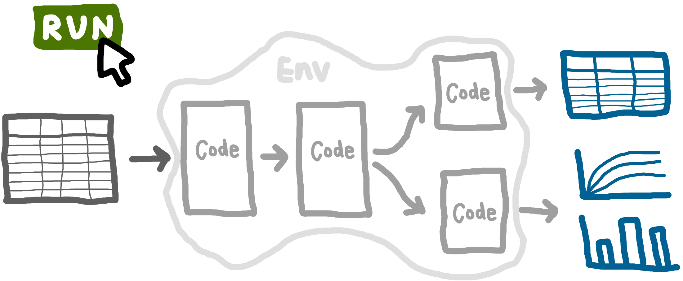
A key aspect RAPs is being able to run your entire analysis from start to finish with a single command. For example, one command that can run a simulation model, evaluate the base case, explore scenarios, conduct sensitivity analyses, and produce all tables and figures.
Why is this important? Running analyses bit by bit makes it easy to introduce inconsistencies. Running everything from scratch ensures that results are fully reproducible: all required code and data are included, and the workflow can be reliably repeated. This means you (or anyone else) can execute the analysis and get all the outputs.
Methods for running everything from scratch
There are several ways to automate running your analysis - some common options include:
main.py: Use if everything is in
.pyfiles (i.e., no Jupyter notebooks). Write a main python function that imports all the necessary code and runs your pipeline.Bash scripts: Can run a mixture of file types (e.g.,
.py,.ipynb,.qmd). You write a shell script that lists each step in your workflow, and the script will execute everything step-by-step in the order you specify.
main.R: Use if everything is in
.Rfiles (i.e., no Rmarkdown files). You create a main script that imports all the necessary code and runs your pipeline.Bash scripts: Can run a mixture of file types (e.g.,
.py,.Rmd,.qmd). You write a shell script that lists each step in your workflow, and the script will execute everything step-by-step in the order you specify.
Makefiles: Handy for analyses with long run times. Makefiles track which outputs depend on which inputs, and only re-run steps when the inputs have changed (i.e., won’t necessarily re-run everything).
Snakemake: Tool that builds on Makefile, supporting very complex pipelines and lots of tools and languages.
In this example, we’ll focus on a bash script, since it’s often the simplest way to run an analysis from scratch and supports a variety of file types.
Bash script
What are bash scripts?
A bash script is a plain text file that contains a list of terminal commands, written for the Bash shell, that are executed in order from top to bottom. Instead of typing each command manually, you save them in a .sh file and run the script to perform the whole sequence with a single command
Where to put the script?
Save the script below as run_notebooks.sh in the project root - for example:
├── run_notebooks.sh
├── notebooks/
|   └── ...
├── simulation/
|   └── ...
├── ...
This allows the script to loop over all .ipynb in the notebooks/ folder using notebooks/*.ipynb without extra path adjustments.
Save the script below as run_rmarkdown.sh in the project root - for example:
├── run_rmarkdown.sh
├── R/
|   └── ...
├── rmarkdown/
|   └── ...
├── ...
This allows the script to loop over all .Rmd files in the rmarkdown/ folder using rmarkdown/*.Rmd without extra path adjustments.
Which terminal to use?
This script is written for Bash.
Linux or macOS users can just use their normal terminal (which runs Bash or a compatible shell).
On Windows, you’ll need to run it from a bash-compatible terminal like Git Bash. PowerShell and Command Prompt use different syntax and cannot run .sh bash scripts directly.
Example script
This example runs Jupyter notebook (.ipynb) files:
#!/usr/bin/env bash

# Get the conda environment's jupyter path
CONDA_JUPYTER=$(dirname "$(which python)")/jupyter

run_notebook() {
    local nb="$1"
    echo "🏃 Running notebook: $nb"
    if "${CONDA_JUPYTER}" nbconvert --to notebook --inplace --execute \
        --ClearMetadataPreprocessor.enabled=True \
        --ClearMetadataPreprocessor.clear_notebook_metadata=True \
        "$nb"
    then
        echo "✅ Successfully processed: $nb"
    else
        echo "❌ Error processing: $nb"
    fi
    echo "-------------------------"
}

if [[ -n "$1" ]]; then
    run_notebook "$1"
else
    for nb in notebooks/*.ipynb; do
        run_notebook "$nb"
    done
fi
Explaining the bash script line by line
#!/usr/bin/env bashThis is called a “shebang line”. It just tells the operating system which interpreter to use - in this case, making sure it uses Bash.
# Get the conda environment's jupyter path
CONDA_JUPYTER=$(dirname "$(which python)")/jupyter
This line finds the jupyter executable linked to your current python environment. This ensures it uses the correct version of Jupyter (i.e., instead of trying to run a system-wide or different environment’s Jupyter).
On Windows, jupyter.exe is usually in the Scripts folder of your conda environment, not directly next to python.exe. For example, if which python returns envs/des-example/python.exe, then jupyter.exe is typically at env/des-example/Scripts/jupyter.exe. You will want to change the line above to:
CONDA_JUPYTER=$(dirname "$(which python)")/Scripts/jupyter`run_notebook() {We define a bash function to run each notebook.
local nb="$1"This assigns the notebook filename passed to the function ($1) to the variable nb within the function.
echo "🏃 Running notebook: $nb"A message is printed to help track what’s happening, as each notebook is processed.
    if "${CONDA_JUPYTER}" nbconvert --to notebook --inplace --execute \
        --ClearMetadataPreprocessor.enabled=True \
        --ClearMetadataPreprocessor.clear_notebook_metadata=True \
        "$nb"
    then
        echo "✅ Successfully processed: $nb"
    else
        echo "❌ Error processing: $nb"
    fi
    echo "-------------------------"
}
This block runs the notebook using Jupyter’s nbconvert tool. It will print a success message if this works, and an error message if not.
The Jupyter nbconvert command (a single command, though split across several lines):
"${CONDA_JUPYTER}" nbconvert: Execute nbconvert from your environment.--to notebook --inplace --execute: Run the notebook, overwrite in place, and execute all cells from scratch.- By using
--inplace, nbconvert overwrites the existing notebook file with the executed version. If you prefer to keep the original notebook and write the executed result to a new file, remove--inplaceand use--output. - You can also change
--to notebookto another format (e.g.,--to htmlgenerates HTML).
- By using
--ClearMetadataPreprocessor.enabled=True: Enable pre-processor that can clear notebook metadata.--ClearMetadataPreprocessor.clear_notebook_metadata=True: Remove notebook metadata."$nb": Specifies the notebook file to run.
if [[ -n "$1" ]]; then
    run_notebook "$1"
else
    for nb in notebooks/*.ipynb; do
        run_notebook "$nb"
    done
fi
If a notebook name is given as a command-line argument, it only runs that notebook. If not, it loops through all notebooks in the notebooks/ directory and runs each one. This structure gives you flexibility: you can run all notebooks in bulk, or just one at a time, without changing the script.
Running the bash script
Make sure your terminal is in the project folder (i.e., the place where run_notebooks.sh is).
# Check where you are
pwd

# List files; you should see run_notebooks.sh and notebooks/
ls
If you are not in the correct folder, use cd path/to/your/project.
To run the script without making it executable:
bash run_notebooks.shTo run a specific notebook:
bash run_notebooks.sh notebooks/notebook_name.ipynbYou can make it executable using chmod +x. This means you can then run it directly (without typing bash first) from anywhere in your project folder tree (i.e., don’t need to be in same directly).
chmod +x run_notebooks.sh
run_notebooks.sh
The output will look like:
> bash run_notebooks.sh notebooks/generate_exp_results.ipynb
🏃 Running notebook: notebooks/generate_exp_results.ipynb
[NbConvertApp] Converting notebook notebooks/generate_exp_results.ipynb to notebook
[NbConvertApp] Writing 35327 bytes to notebooks/generate_exp_results.ipynb
✅ Successfully processed: notebooks/generate_exp_results.ipynb
-------------------------
Including .py files in the bash script
Our example script just ran Jupyter notebooks, as they contained all our analysis in our example models. However, you can also perform your analysis in .py files, structured like:
from simulation import Param, Runner


def main():
    runner = Runner(param = Param())
    runner.run_reps()
    # Continues to analysis and saves outputs...


if __name__ == "__main__":
    main()
These can then be easily run from the command line:
python filename.pyYou could put your whole pipeline inside a single main() function and avoid bash scripts altogether. However, a separate bash script becomes useful when you want to mix different tools (e.g., .ipynb and .py) and languages in one pipeline.
#!/bin/bash

# Ensure the script exits on error
set -e

# Find and render all .Rmd files in the specified directory
for file in "rmarkdown"/*.Rmd; do
    echo "Rendering: $file"
    Rscript -e "rmarkdown::render('$file')"
done

echo "Rendering complete!"
It starts with #!/usr/bin/env bash. This is known as a “shebang line”. It just tells the operating system which interpreter to use - in this case, making sure it uses Bash.
It is set to end on error running any file (set -e).
It searches for every file ending .Rmd in the rmarkdown folder. For each file, it prints a message to say which file it is working on (echo ...), and then runs R code to execute the file.
Running the bash script
To run the script, open a terminal and run:
bash run_rmarkdown.shYou can make it executable using chmod +x. You can then run it directly (without typing bash first) from anywhere in your project folder tree (i.e., don’t need to be in same directly).
chmod +x run_rmarkdown.sh
run_rmarkdown.sh
The output of running the script will look something like this:
> bash run_rmarkdown.sh
Rendering: rmarkdown/analysis.Rmd


processing file: analysis.Rmd
  |....................                               |  39% [unnamed-chunk-9]
Including .R files in the bash script.
Our example script just ran rmarkdown files, as they contained all our analysis in our example models. However, you can also perform your analysis in .R files, structured like:
devtools::load_all()

run_results <- runner(param = parameters())[["run_results"]]
# Continues with analysis and saving outputs...
You can run this R script from a Bash script or terminal with the following command:
Rscript analysis/filename.RYou could call your whole pipeline from inside a single R script and avoid bash scripts altogether. However, a separate bash script becomes useful when you want to mix different tools (e.g., .Rmd and R files) and languages in one pipeline.
Literate programming
Literate programming is an approach where code and narrative text are combined in a single document. For example, using Jupyter notebooks (.ipynb) or Quarto files (.qmd).
Literate programming is an approach where code and narrative text are combined in a single document. For example, using Rmarkdown files (.Rmd) or Quarto files (.qmd).
This style of working can be really handy for reproducibility, as all the parameter choices, steps and outputs are documented alongside explanatory text.
There are several common ways to use literate programming in research workflows:
Experimentation - treating the documents like digital lab books, they contain all the analysis and experiments, with the final write-up kept separate.
Write-up with dynamic outputs - pre-generated outputs (figures, tables, statistics) are dynamically embedded in the write-up document, so that results remain accurate and up-to-date. This set-up allows analysis and reporting to be updated/run consecutively or independently.
Code-integrated manuscripts (“reproducible manuscripts”) - the full analysis (including code to run models) lives inside the write-up. Depending on the intended audience, code chunks may be shown or hidden.
Literate programming documents can be styled for journal or pre-print formats, making them suitable for publication submissions. Some handy resources (including Python and R versions, as though sometimes language-specific, both can be handy for the other):
- “Writing Reproducible Manuscripts in R & Python” from Research Data Management Support at Utrecht University (2025).
- “Reproducible Manuscripts” from Stanford Psychology Guide to Doing Open Science (2020).
- “Writing a reproducible paper with RStudio and Quarto” from Bauer, P. C., and Landesvatter, C. (2023).
- “Writing a reproducible paper with R Markdown and Pagedown” from Bauer, P. C., and Landesvatter, C. (2021).
Explore the example models
![]() Click to visit pydesrap_mms repository
Click to visit pydesrap_mms repository
![]() Click to visit pydesrap_stroke repository
Click to visit pydesrap_stroke repository
Both have a file run_notebooks.sh (like the example above) which is used to run everything in notebooks/ from scratch.
![]() Click to visit rdesrap_mms repository
Click to visit rdesrap_mms repository
![]() Click to visit rdesrap_stroke repository
Click to visit rdesrap_stroke repository
Both have a file run_rmarkdown.sh (like the example above) which is used to run everything in rmarkdown/ from scratch.
Test yourself
Quiz
run_notebooks.sh?
run_rmarkdown.sh?
Activity
Try writing a bash scripts that runs some of your analysis files.
You can print a message before running each one to check whether each command succeeded.
Use a loop to run all the files in a given directory.