Time-dependent arrivals

1. Background

The treatment simulation model has a time-dependent arrival profile for patients. To simulated these arrivals correctly in DES we need to use one of several algorithms. Here we make use of the thinning algorithm.

Thinning is a acceptance-rejection sampling method and is used to generate inter-arrival times from a NSPP.

Motivation: In DES we use thinning as an approach to generate time dependent arrival of patients to a health care service.

1.1 An example NSPP

The table below is adapted from Banks et al (2013) and breaks an arrival process down into 60 minutes intervals.

t(min)	Mean time between arrivals (min)	Arrival Rate \(\lambda(t)\) (arrivals/min)
0	15	1/15
60	12	1/12
120	7	1/7
180	5	1/5
240	8	1/8
300	10	1/10
360	15	1/15
420	20	1/20
480	20	1/20

Interpretation: In the table above the fastest arrival rate is 1/5 customers per minute or 5 minutes between patient arrivals.

1.2 The thinning algorithm

A NSPP has arrival rate \(\lambda(t)\) where \(0 \leq t \leq T\)

Here \(i\) is the arrival number and \(\mathcal{T_i}\) is its arrival time.

1. Let \(\lambda^* = \max_{0 \leq t \leq T}\lambda(t)\) be the maximum of the arrival rate function and set \(t = 0\) and \(i=1\)

2. Generate \(e\) from the exponential distribution with rate \(\lambda^*\) and let \(t = t + e\) (this is the time of the next entity will arrive)

3. Generate \(u\) from the \(U(0,1)\) distribution. If \(u \leq \dfrac{\lambda(t)}{\lambda^*}\) then \(\mathcal{T_i} =t\) and \(i = i + 1\)

4. Go to Step 2.

2. Imports

library(simmer)
library(tibble)
library(ggplot2)
suppressMessages(library(RCurl))

3. Read in data

Here we read in the example non-stationary data and compute the arrival rate.

NSPP_PATH = 'https://raw.githubusercontent.com/TomMonks/treat-sim-rsimmer/main/data/nspp_example1.csv'

csv_data <- getURL(NSPP_PATH)
arrivals <- read.csv(text=csv_data)
names(arrivals) <- c("period", "mean_iat")

# create arrival rate
arrivals$arrival_rate = 1.0 / arrivals$mean_iat

arrivals

  period mean_iat arrival_rate
1      0       15   0.06666667
2     60       12   0.08333333
3    120        7   0.14285714
4    180        5   0.20000000
5    240        8   0.12500000
6    300       10   0.10000000
7    360       15   0.06666667
8    420       20   0.05000000
9    480       20   0.05000000

ggplot(data=arrivals, aes(x=period, y=mean_iat)) +
  geom_bar(stat="identity", fill="steelblue") + 
  xlab("Time of day (mins)") + 
  ylab("Mean IAT (min)")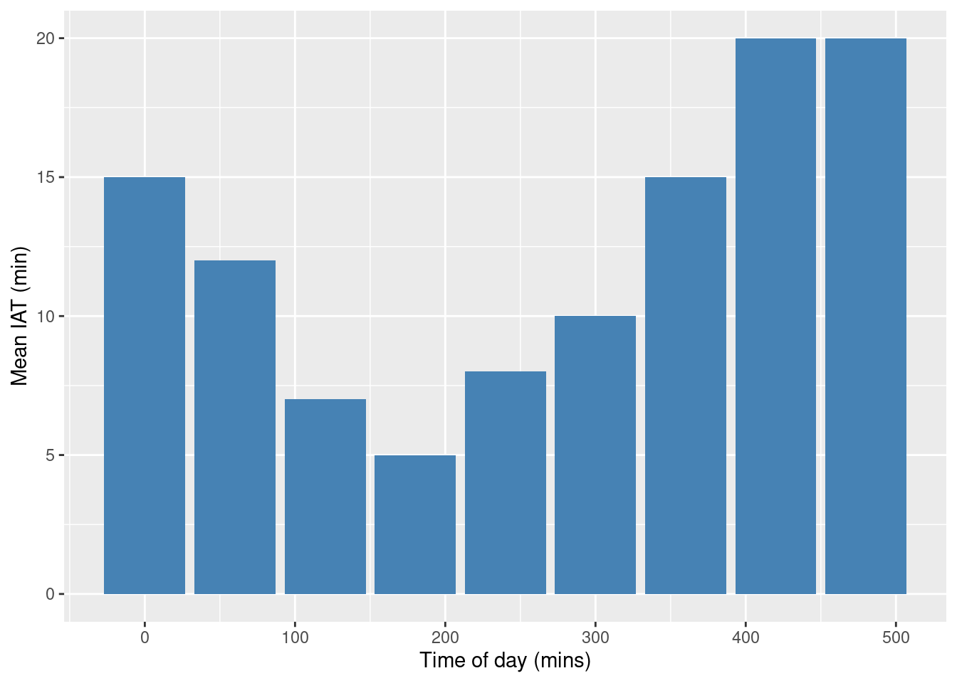

4. Algorithm implementation

4.1 NSPP sampling function

nspp_thinning <- function(simulation_time, data, debug=FALSE){
  
  # calc time interval: assumes intervals are of equal length
  interval <- data$period[2] - data$period[1]
  
  # maximum arrival rate (smallest time between arrivals)
  lambda_max <- max(data$arrival_rate)

  while(TRUE){
    # get time bucket (row of dataframe to use)
    t <- floor(simulation_time / interval) %% nrow(data) + 1
    lambda_t <- data$arrival_rate[t]
    
    # set to a large number so that at least 1 sample is taken
    u <- Inf
    rejects <- -1
    
    # running total of time until next arrival
    inter_arrival_time <- 0.0
    
    # reject proportionate to lambda_t / lambda_max
    ratio <- lambda_t / lambda_max
    while(u >= ratio){
      rejects <- rejects + 1
      # sample using max arrival rate
      inter_arrival_time <- inter_arrival_time + rexp(1, lambda_max)
      u <- runif(1, 0.0, 1.0)
    }
    
    if(debug){
      print({paste("Time:", simulation_time, 
                   " Rejections:", rejects, 
                   " t:", t, 
                   " lambda_t:", lambda_t, 
                   " IAT:", inter_arrival_time)})
    }
      
    return(inter_arrival_time)
  }
}

4.2 Example usage

The function can be used in the same way as rexp to generate new patients. To illustrate its use we first create a simple patient pathway trajectory that prints out some event and acts as a delay.

patient <- trajectory("patient pathway") %>% 
  # just a simple delay
  log_(function() {paste("Patient arrival")}, level = 1) %>% 
  timeout(function() rnorm(1, 10.0, 1.0)) %>% 
  log_(function() {paste("Exit treatment pathway")}, level = 1)

We then run the model with a generator that uses the nspp_thinning sampling function. Note that the function accepts the current simulation time now(env) and the dataframe containing the arrivals arrivals.

Important learning point: we need to detach run from the creation of the simulation environment. This will allow now(env) to run correctly. If we ignore this rule and include run in the creation pipe the same time will be passed to the thinning function and it will under/over sample arrivals. See https://r-simmer.org/articles/simmer-03-trajectories.html

env <- simmer("TreatSim", log_level=0) 

env %>% 
  add_generator("patient", patient, 
                function() nspp_thinning(now(env), arrivals, debug=TRUE)) %>% 
  run(until=540.0)

[1] "Time: 0  Rejections: 2  t: 1  lambda_t: 0.0666666666666667  IAT: 12.3170700045055"
[1] "Time: 12.3170700045055  Rejections: 2  t: 1  lambda_t: 0.0666666666666667  IAT: 29.8042921362527"
[1] "Time: 42.1213621407582  Rejections: 4  t: 1  lambda_t: 0.0666666666666667  IAT: 44.3244025730205"
[1] "Time: 86.4457647137787  Rejections: 0  t: 2  lambda_t: 0.0833333333333333  IAT: 1.5125033070694"
[1] "Time: 87.9582680208481  Rejections: 1  t: 2  lambda_t: 0.0833333333333333  IAT: 4.80466362067914"
[1] "Time: 92.7629316415272  Rejections: 0  t: 2  lambda_t: 0.0833333333333333  IAT: 2.07653273129836"
[1] "Time: 94.8394643728255  Rejections: 1  t: 2  lambda_t: 0.0833333333333333  IAT: 12.7656335775265"
[1] "Time: 107.605097950352  Rejections: 1  t: 2  lambda_t: 0.0833333333333333  IAT: 6.69238817158571"
[1] "Time: 114.297486121938  Rejections: 3  t: 2  lambda_t: 0.0833333333333333  IAT: 11.4083337817366"
[1] "Time: 125.705819903674  Rejections: 0  t: 3  lambda_t: 0.142857142857143  IAT: 0.232516925316304"
[1] "Time: 125.938336828991  Rejections: 1  t: 3  lambda_t: 0.142857142857143  IAT: 6.2632446431317"
[1] "Time: 132.201581472122  Rejections: 0  t: 3  lambda_t: 0.142857142857143  IAT: 1.50837458437309"
[1] "Time: 133.709956056495  Rejections: 0  t: 3  lambda_t: 0.142857142857143  IAT: 3.85685536989427"
[1] "Time: 137.56681142639  Rejections: 2  t: 3  lambda_t: 0.142857142857143  IAT: 20.6832564180142"
[1] "Time: 158.250067844404  Rejections: 0  t: 3  lambda_t: 0.142857142857143  IAT: 6.35431296636766"
[1] "Time: 164.604380810772  Rejections: 3  t: 3  lambda_t: 0.142857142857143  IAT: 45.955617979437"
[1] "Time: 210.559998790209  Rejections: 0  t: 4  lambda_t: 0.2  IAT: 1.42062998576036"
[1] "Time: 211.980628775969  Rejections: 0  t: 4  lambda_t: 0.2  IAT: 0.458430694988776"
[1] "Time: 212.439059470958  Rejections: 0  t: 4  lambda_t: 0.2  IAT: 5.25860620175904"
[1] "Time: 217.697665672717  Rejections: 0  t: 4  lambda_t: 0.2  IAT: 4.17272278086698"
[1] "Time: 221.870388453584  Rejections: 0  t: 4  lambda_t: 0.2  IAT: 0.229960032738745"
[1] "Time: 222.100348486322  Rejections: 0  t: 4  lambda_t: 0.2  IAT: 0.652627080552088"
[1] "Time: 222.752975566875  Rejections: 0  t: 4  lambda_t: 0.2  IAT: 6.63534692933268"
[1] "Time: 229.388322496207  Rejections: 0  t: 4  lambda_t: 0.2  IAT: 5.01297508811063"
[1] "Time: 234.401297584318  Rejections: 0  t: 4  lambda_t: 0.2  IAT: 2.69523442257196"
[1] "Time: 237.09653200689  Rejections: 0  t: 4  lambda_t: 0.2  IAT: 2.71995460847393"
[1] "Time: 239.816486615364  Rejections: 0  t: 4  lambda_t: 0.2  IAT: 5.35320844014591"
[1] "Time: 245.16969505551  Rejections: 1  t: 5  lambda_t: 0.125  IAT: 6.91582239444783"
[1] "Time: 252.085517449958  Rejections: 0  t: 5  lambda_t: 0.125  IAT: 6.39692617551118"
[1] "Time: 258.482443625469  Rejections: 1  t: 5  lambda_t: 0.125  IAT: 33.31127954999"
[1] "Time: 291.793723175459  Rejections: 0  t: 5  lambda_t: 0.125  IAT: 6.32686956764615"
[1] "Time: 298.120592743105  Rejections: 0  t: 5  lambda_t: 0.125  IAT: 0.6473648018442"
[1] "Time: 298.767957544949  Rejections: 0  t: 5  lambda_t: 0.125  IAT: 0.562435596448654"
[1] "Time: 299.330393141398  Rejections: 0  t: 5  lambda_t: 0.125  IAT: 14.3972218773308"
[1] "Time: 313.727615018728  Rejections: 0  t: 6  lambda_t: 0.1  IAT: 4.03505245840212"
[1] "Time: 317.762667477131  Rejections: 0  t: 6  lambda_t: 0.1  IAT: 12.9321964642472"
[1] "Time: 330.694863941378  Rejections: 0  t: 6  lambda_t: 0.1  IAT: 8.29896487253618"
[1] "Time: 338.993828813914  Rejections: 1  t: 6  lambda_t: 0.1  IAT: 4.86410341841185"
[1] "Time: 343.857932232326  Rejections: 1  t: 6  lambda_t: 0.1  IAT: 8.14657132614103"
[1] "Time: 352.004503558467  Rejections: 1  t: 6  lambda_t: 0.1  IAT: 5.96838979960835"
[1] "Time: 357.972893358075  Rejections: 0  t: 6  lambda_t: 0.1  IAT: 0.566974185257226"
[1] "Time: 358.539867543332  Rejections: 2  t: 6  lambda_t: 0.1  IAT: 17.9213087428416"
[1] "Time: 376.461176286174  Rejections: 2  t: 7  lambda_t: 0.0666666666666667  IAT: 7.19756458909887"
[1] "Time: 383.658740875273  Rejections: 7  t: 7  lambda_t: 0.0666666666666667  IAT: 28.6240846114835"
[1] "Time: 412.282825486756  Rejections: 7  t: 7  lambda_t: 0.0666666666666667  IAT: 37.641882830785"
[1] "Time: 449.924708317541  Rejections: 0  t: 8  lambda_t: 0.05  IAT: 6.7952759422124"
[1] "Time: 456.719984259754  Rejections: 1  t: 8  lambda_t: 0.05  IAT: 6.45498812368717"
[1] "Time: 463.174972383441  Rejections: 2  t: 8  lambda_t: 0.05  IAT: 12.2225909600384"
[1] "Time: 475.397563343479  Rejections: 0  t: 8  lambda_t: 0.05  IAT: 11.025298134725"
[1] "Time: 486.422861478204  Rejections: 5  t: 9  lambda_t: 0.05  IAT: 14.8031513880246"
[1] "Time: 501.226012866229  Rejections: 0  t: 9  lambda_t: 0.05  IAT: 7.47590314554882"
[1] "Time: 508.701916011778  Rejections: 5  t: 9  lambda_t: 0.05  IAT: 36.0732168012259"

simmer environment: TreatSim | now: 540 | next: 544.775132813004
{ Monitor: in memory }
{ Source: patient | monitored: 1 | n_generated: 52 }

5. Validation

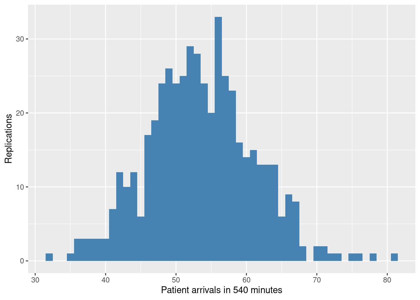
The total number of arrivals in 540 minutes

Here we will repeat the same 10,000 times and then explore the distribution of the number of arrivals. If all has gone to plan this should be a Poisson distribution with mean ~53.

# expected arrivals from data.
round(sum(arrivals$arrival_rate * 60), 2)

[1] 53.07

We can use the simmer function get_n_generated to return the number of patients generated.

arrivals_by_replication <- function(envs){
  results <- vector()
  for(env in envs){
    results <- c(results, get_n_generated(env, "patient"))
  }
  return(data.frame(results))
}

single_run <- function(env, rep_number, run_length, debug_arrivals=FALSE){
  env %>% 
    add_generator("patient", patient, 
                  function() nspp_thinning(now(env), arrivals, debug=debug_arrivals)) %>% 
    run(until=540.0)
  return(env)
}

RUN_LENGTH <- 540.0
N_REPS <- 500
SEED <- 42

set.seed(SEED)

patient <- trajectory("patient pathway") %>% 
  # just a simple delay
  log_(function() {paste("Exit treatment pathway")}, level = 1)

# note unlike in simmer documentation we use a traditional for loop
# instead of lapply. This allows us to separeate env creation
# from run and preserve the environment interaction between NSPP 
# and current sim time.
envs = vector()
for(rep in 1:N_REPS){
  env <- simmer("TreatSim", log_level=0) 
  single_run(env, i, RUN_LENGTH)
  envs <- c(envs, env)
}

# # get the number of arrivals generated
results <- arrivals_by_replication(envs)

# show mean number of arrivals. Should be close to 53
mean(results$results)

[1] 53.552

ggplot(results, aes(x=results)) + 
  geom_histogram(binwidth=1, fill="steelblue") + 
  xlab("Patient arrivals in 540 minutes") + 
  ylab("Replications")