Stroke+Rehab models

import pandas as pd
import numpy as np

Model outputs

The results of the two generated simulations models were identical to 2 decimal places. The results for stage 1 and stage 2 models are reported and compared graphically below in Fig. 8 and Fig. 9. The figures show that the probability of delay and ward occupancy match across the acute and rehabilitation wards within the 2 models.

The outputs from the generated models results replicated the results reported in the original article [Monks et al., 2016]; although we note that did not run all of the experiments reported in the article.

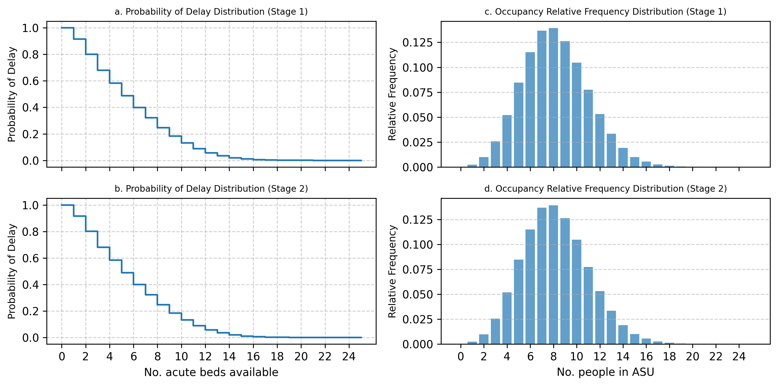
Fig. 8 Acute stroke unit outputs: comparison of stage 1 and stage 2 models

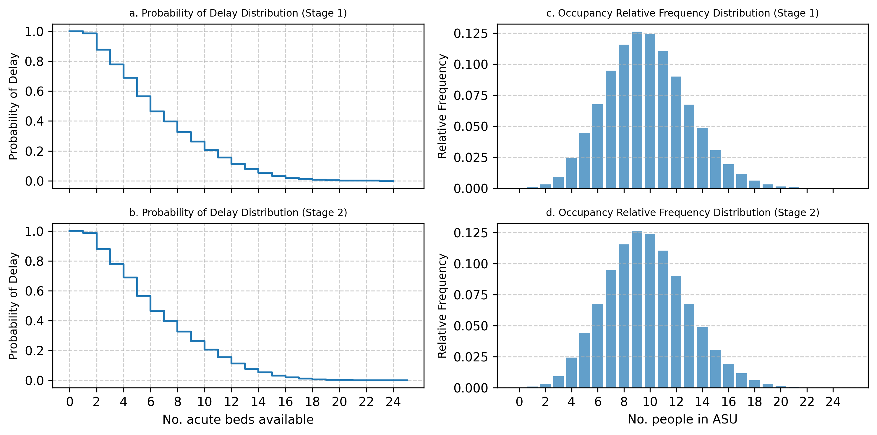
Fig. 9 Rehabilitation unit outputs: comparison of stage 1 and stage 2 models

Model code

The final code files from stage 1 and stage 2 (our internal replication) for the stroke capacity planning model have some substantial differences. The table below summarises the difference in implementation. Notable differences included an additional PatientType class in the stage 2 model; and a six-fold difference in the number of member attributes of the Experiment class. This latter result is somewhat misleading as the same number of model parameters are settable in both models. The difference is due to the stage 2 generated code making use of a different data structure (we discuss this below regarding difference in the the setup and use of models).

Disregarding comments, documentation and the streamlit interface, stage 1 generated a simpy model consisting of 436 line of code and stage 2 generated 531 lines of code. Both models passed the same batch of 34 verification tests.

Component	Number of Attributes (Stage 1)	Number of Attributes (Stage 2)	Number of Methods/Functions (Stage 1)	Number of Methods/Functions (Stage 2)
Experiment class	36	5	3	5
PatientType class	N/A	6	N/A	3
AcuteStrokeUnit model logic class	5	7	6	7
RehabilitationUnit model logic class	6	18	7	9
Functions (excluding classes)	N/A	N/A	11	10

Table: Count of stroke capacity planning model code components comparing Stages 1 and 2.

Complexity of setup and use of models

Although the stage 1 and 2 models produced identical outputs the internal implementation of the Experiment class varied substantially. The code generated by the LLM led to quite different interfaces to setup and create an instance of Experiment and then to access internal parameters.

For example, in the stage 1 model the code to setup an experiment that simulated a 5% increase in stroke patients, and then check the parameter value was as follows:

# setup experiment
default_experiment = Experiment(stroke_mean=1.2*1.05)

# access and check parameter value
print(default_experiment.stroke_mean)

The equivalent code in stage 2 involved an additional line of code to create a experimentation dictionary and a collection data-structure approach to access the internal parameters.

# setup paramater dictionary
experiment_params = {"patient_types": {"Stroke": {"interarrival_time": 1.2 * 1.05}}}

# pass to Experiment. LLM provided code that updates internal parameter dictionaries
future_demand_experiment = Experiment(experiment_params)

# access and check parameter value
print(future_demand_experiment.params['patient_types']['Stroke']['interarrival_time'])

We do not argue that either of the approaches generated by the LLM is optimal. Rather that there are pro’s and con’s to their implementations. Stage 1 code offers a simple interface, but does not choose a clear naming convention (stroke_mean is not specific to inter-arrival time). Stage 1 also does not clearly separate model parameters from the outputs of the experiment. Stage 2 code requires more code and requires a user to understand Python dictionaries. Stage 2’s hierarchy to access parameters is more complex than stage 1’s (including the internal workings of Experiment), but it uses clear specific naming conventions for patients types and their different parameters configurations.

streamlit interfaces

The model interfaces were very similar and are depicted in Fig. 10 and Fig. 11. The main difference in the interface code generated related to input widgets used to manipulate model input parameters. In stage 1 “numeric boxes” were used where-as in stage 2 “sliders” are used. The former allowed the input parameters to take negative values - that result in a model error (as you cannot have a negative inter-arrival arrival rate) - where-as sliders prevented this unacceptable setting with a minimum value (although still allowed 0).

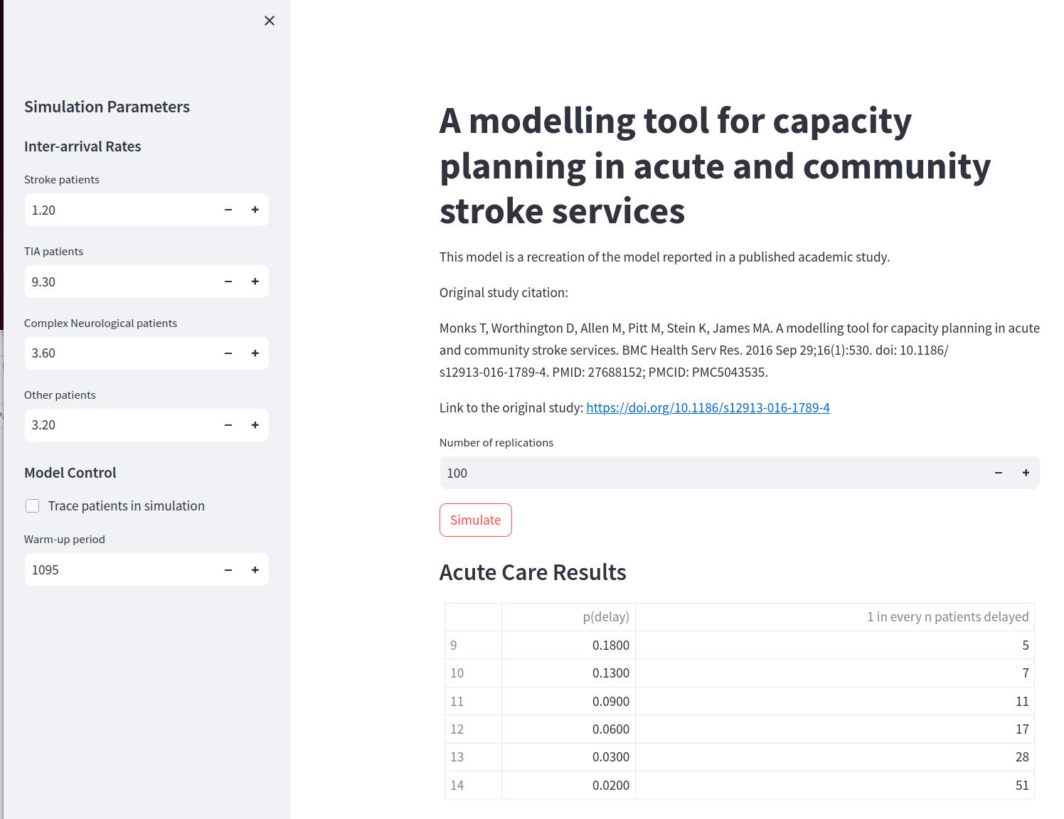
Fig. 10 Stroke+Rehab model interface generated in Stage 1.

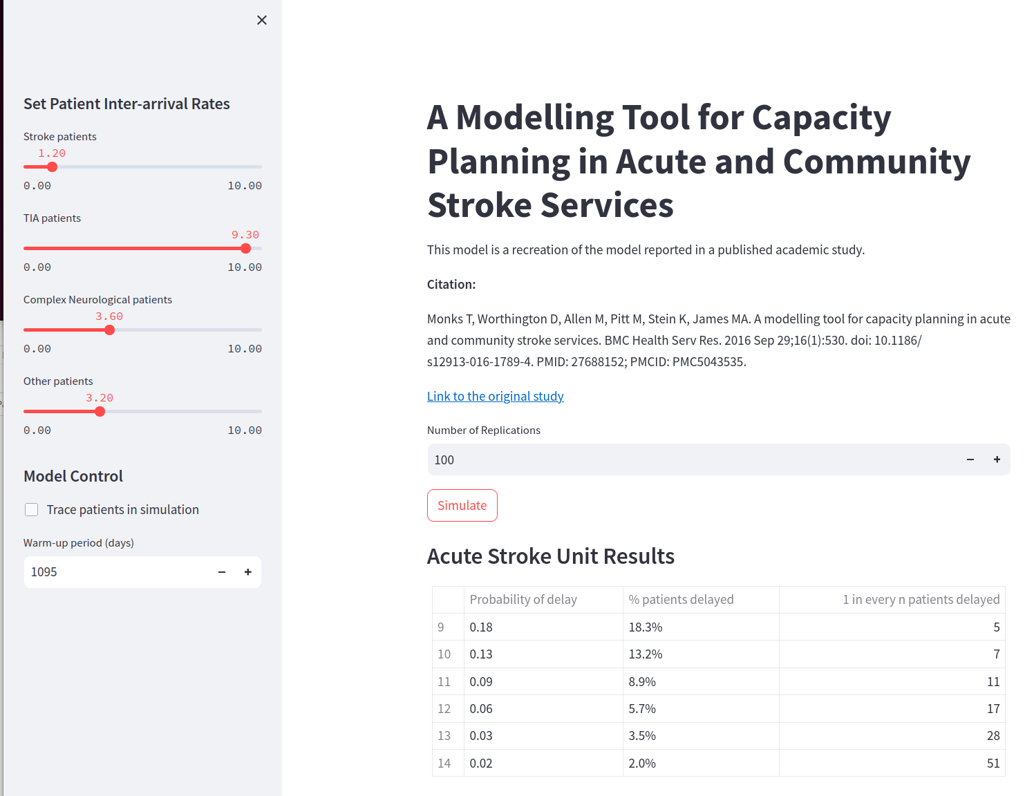
Fig. 11 Stroke+Rehab model interface generated in Stage 2.

Lines of code data

!pygount --suffix=py --format=summary ../../03_stroke/stroke_rehab_model.py

?25l
Working... ━━━━━━━━━━━━━━━━━━━━━━━━━━━━━━━━━━━━━━━━   0% -:--:--

Working... ━━━━━━━━━━━━━━━━━━━━━━━━━━━━━━━━━━━━━━━━   0% -:--:--

Working... ━━━━━━━━━━━━━━━━━━━━━━━━━━━━━━━━━━━━━━━━   0% -:--:--

Working... ━━━━━━━━━━━━━━━━━━━━━━━━━━━━━━━━━━━━━━━━ 100% 0:00:00
Working... ━━━━━━━━━━━━━━━━━━━━━━━━━━━━━━━━━━━━━━━━ 100% 0:00:00
?25h
┏━━━━━━━━━━┳━━━━━━━┳━━━━━━━┳━━━━━━┳━━━━━━┳━━━━━━━━━┳━━━━━━┓
┃ Language ┃ Files ┃     % ┃ Code ┃    % ┃ Comment ┃    % ┃
┡━━━━━━━━━━╇━━━━━━━╇━━━━━━━╇━━━━━━╇━━━━━━╇━━━━━━━━━╇━━━━━━┩
│ Python   │     1 │ 100.0 │  436 │ 55.2 │     188 │ 23.8 │
├──────────┼───────┼───────┼──────┼──────┼─────────┼──────┤
│ Sum      │     1 │ 100.0 │  436 │ 55.2 │     188 │ 23.8 │
└──────────┴───────┴───────┴──────┴──────┴─────────┴──────┘

# code for stroke
# !pygount --suffix=py --format=summary ../../03_stroke/stroke_rehab_model.py
# !pygount --suffix=py --format=summary ../../03_stroke/stroke_rehab_interface.py

!pygount --suffix=py --format=summary ../../03_stroke/s2_stroke_rehab_model.py

?25l
Working... ━━━━━━━━━━━━━━━━━━━━━━━━━━━━━━━━━━━━━━━━   0% -:--:--

Working... ━━━━━━━━━━━━━━━━━━━━━━━━━━━━━━━━━━━━━━━━   0% -:--:--

Working... ━━━━━━━━━━━━━━━━━━━━━━━━━━━━━━━━━━━━━━━━   0% -:--:--

Working... ━━━━━━━━━━━━━━━━━━━━━━━━━━━━━━━━━━━━━━━━   0% -:--:--
Working... ━━━━━━━━━━━━━━━━━━━━━━━━━━━━━━━━━━━━━━━━ 100% 0:00:00
Working... ━━━━━━━━━━━━━━━━━━━━━━━━━━━━━━━━━━━━━━━━ 100% 0:00:00
?25h
┏━━━━━━━━━━┳━━━━━━━┳━━━━━━━┳━━━━━━┳━━━━━━┳━━━━━━━━━┳━━━━━┓
┃ Language ┃ Files ┃     % ┃ Code ┃    % ┃ Comment ┃   % ┃
┡━━━━━━━━━━╇━━━━━━━╇━━━━━━━╇━━━━━━╇━━━━━━╇━━━━━━━━━╇━━━━━┩
│ Python   │     1 │ 100.0 │  531 │ 64.6 │      74 │ 9.0 │
├──────────┼───────┼───────┼──────┼──────┼─────────┼─────┤
│ Sum      │     1 │ 100.0 │  531 │ 64.6 │      74 │ 9.0 │
└──────────┴───────┴───────┴──────┴──────┴─────────┴─────┘

Prompts

In total 31 iterations of the model were used to build the model and interface. In stage 1 this consisted of 41 prompts passed to the LLM. The number of prompts increased to 57 in stage 2. In total n (TO-DO) additional prompts were needed in stage 2 to fix a variable type bug introduced by the LLM for representing “patient type” across the acute and rehab sections of the model. Stage 2 required 4 additional prompts for introducing common random numbers streams to the LLM struggling to assign streams across model activities (TO-do: check with Alison).

The table below provides a summary of the differences at each iteration.

def highlight_last_row(df: pd.DataFrame) -> list[str]:
    '''
    highlight the last row (for Totals) in a DataFrame in BOLD.
    
    Source:
    -------

    Adapted from stackoverflow
    https://stackoverflow.com/questions/51938245/display-dataframe
    -values-in-bold-font-in-one-row-only#59493062
    '''
    return ['font-weight: bold' if v == df.iloc[-1] else '' for v in df]

# read in prompt results table
prompt_results = (
    pd.read_csv("data/stroke_prompt_table.csv",
                index_col=['Iteration'])
)

prompt_results.loc[len(prompt_results) + 1] = ["Totals"] + prompt_results.sum().tolist()[-3:]
prompt_results.style.apply(highlight_last_row)

	Added functionality	Stage 1	Stage 2	Difference
Iteration
1	Acute stroke unit (ASU) arrivals	1	3	2
2	Sample post stroke unit destination	1	1	0
3	Acute stroke unit length of stay (1)	1	2	1
4	Acute stroke unit length of stay (2)	1	1	0
5	Organise parameters	1	1	0
6	Track ASU bed occupancy	1	1	0
7	Functionality to suppress simulation event log	2	2	0
8	ASU results collection functionality	1	2	1
9	ASU occupancy plot	1	1	0
10	ASU probability of delay	1	1	0
11	Bug fix: add back in code that was removed by LLM	1	0	-1
12	Rehab external arrivals	1	1	0
13	Organise parameters	2	2	0
14	Rehab unit length of stay (1)	1	1	0
15	Organise parameters	2	3	1
16	Rehab unit length of stay (2)	1	1	0
17	Track Rehab unit bed occupancy	1	1	0
18	Rehab unit results collection functionality	2	2	0
19	Link ASU and Rehab models (1)	1	1	0
20	Link ASU and Rehab models (2)	2	6	4
21	Warm-up period	2	5	3
22	Multiple replications (1)	1	1	0
23	Multiple replications (2)	1	2	1
24	Common random numbers (1)	1	1	0
25	Common random numbers (2)	1	1	0
26	Common random numbers (3)	2	5	3
27	Common random numbers (4)	2	2	0
28	Model interface (1)	1	1	0
29	Model interface (2)	1	2	1
30	Model interface (3)	1	1	0
31	Bug fix	3	3	0
32	Totals	41	57	16

LateX for manuscript

caption = "The number of prompts given to the LLM " \
          + "at each iteration of the stroke capacity planning model)."
                
print(prompt_results.style.to_latex(caption=caption))

\begin{table}
\caption{The number of prompts given to the LLM at each iteration of the stroke capacity planning model).}
\begin{tabular}{llrrr}
 & Added functionality & Stage 1 & Stage 2 & Difference \\
Iteration &  &  &  &  \\
1 & Acute stroke unit (ASU) arrivals & 1 & 3 & 2 \\
2 & Sample post stroke unit destination & 1 & 1 & 0 \\
3 & Acute stroke unit length of stay (1) & 1 & 2 & 1 \\
4 & Acute stroke unit length of stay (2) & 1 & 1 & 0 \\
5 & Organise parameters & 1 & 1 & 0 \\
6 & Track ASU bed occupancy & 1 & 1 & 0 \\
7 & Functionality to suppress simulation event log & 2 & 2 & 0 \\
8 & ASU results collection functionality & 1 & 2 & 1 \\
9 & ASU occupancy plot & 1 & 1 & 0 \\
10 & ASU probability of delay & 1 & 1 & 0 \\
11 & Bug fix: add back in code that was removed by LLM & 1 & 0 & -1 \\
12 & Rehab external arrivals & 1 & 1 & 0 \\
13 & Organise parameters & 2 & 2 & 0 \\
14 & Rehab unit length of stay (1) & 1 & 1 & 0 \\
15 & Organise parameters & 2 & 3 & 1 \\
16 & Rehab unit length of stay (2) & 1 & 1 & 0 \\
17 & Track Rehab unit bed occupancy & 1 & 1 & 0 \\
18 & Rehab unit results collection functionality & 2 & 2 & 0 \\
19 & Link ASU and Rehab models (1) & 1 & 1 & 0 \\
20 & Link ASU and Rehab models (2) & 2 & 6 & 4 \\
21 & Warm-up period & 2 & 5 & 3 \\
22 & Multiple replications (1) & 1 & 1 & 0 \\
23 & Multiple replications (2) & 1 & 2 & 1 \\
24 & Common random numbers (1) & 1 & 1 & 0 \\
25 & Common random numbers (2) & 1 & 1 & 0 \\
26 & Common random numbers (3) & 2 & 5 & 3 \\
27 & Common random numbers (4) & 2 & 2 & 0 \\
28 & Model interface (1) & 1 & 1 & 0 \\
29 & Model interface (2) & 1 & 2 & 1 \\
30 & Model interface (3) & 1 & 1 & 0 \\
31 & Bug fix & 3 & 3 & 0 \\
32 & Totals & 41 & 57 & 16 \\
\end{tabular}
\end{table}

References

[1]

Thomas Monks, David Worthington, Michael Allen, Martin Pitt, Ken Stein, and Martin A. James. A modelling tool for capacity planning in acute and community stroke services. BMC Health Services Research, 16:530, 2016. doi:10.1186/s12913-016-1789-4.